This page describes how to generate and run a Monte Carlo analysis using script commands. The Monte Carlo analysis tool allows users to run extensive Monte Carlo analysis, sweeping across multiple parameters. This can be useful for assessing statistical variations of circuit elements on overall circuit performance, as well as the effects of variations in component-level simulations. The same example used in the section "Monte Carlo analysis" will be re-generated in this page. For additional information and detailed implementation of the script commands, please see the "Measurement and optimization data" section. Please note that, all the script commands used in this example could also be applied to sweep and optimization analyses.
To generate and run the Monte Carlo analysis using script commands, user can open the run_monte_carlo.icp file and follow the three steps listed below; or, open and run the script file run_monte_carlo_script.lsf .
In this article:
Creating the Monte Carlo analysis
The following commands are used to generate and superficially define a new Monte Carlo analysis named "MC_script".
addsweep(2);
MC_name = "MC_script";
setsweep("Monte Carlo analysis", "name", MC_name);
setsweep(MC_name, "number of trials", 50);
setsweep(MC_name, "enable seed", 1);
setsweep(MC_name, "seed", 1);
setsweep(MC_name, "Variation", "Both");
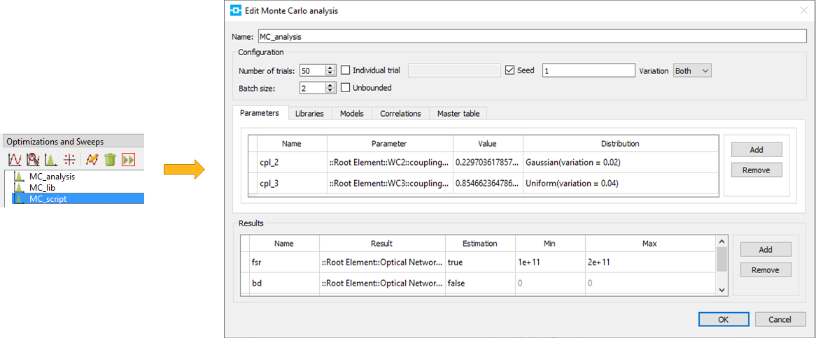
After the Monte Carlo analysis object is superficially generated, the parameters can then be defined and added to it. The following commands define two coupling coefficient parameters (cpl_2 and cpl_3) and add them to the Monte Carlo analysis object "MC_script" in the "Parameters" tab.
# define the parameter cpl
setsweep(MC_name, "type", "Parameters");
cpl2 = struct;
cpl2.Name = "cpl_2";
cpl2.Parameter = "::Root Element::WC2::coupling coefficient 1";
cpl2.Value = getnamed("WC2", "coupling coefficient 1");
dis = struct;
dis.type = "gaussian";
dis.variation = 0.02;
cpl2.Distribution = dis;

cpl3 = struct;
cpl3.Name = "cpl_3";
cpl3.Parameter = "::Root Element::WC3::coupling coefficient 1";
cpl3.Value = getnamed("WC3", "coupling coefficient 1");
dis = struct;
dis.type = "uniform";
dis.variation = 0.04;
cpl3.Distribution = dis;

addsweepparameter(MC_name, cpl2);
addsweepparameter(MC_name, cpl3);
The following commands define the model variation for the waveguide models and the variation is on the group index. This model is added to the "Models" tab.
# define the model ng
wgd_model = struct;
wgd_model.Name = "wgd_model";
wgd_model.Model = "WGD::group index 1";
wgd_model.Value = getnamed("SW1", "group index 1");
global = struct;
global.type = "uniform";
global.variation = 1.02;
wgd_model.Global = global;

local = struct;
local.type = "gaussian";
local.variation = 0.1;
wgd_model.Local= local;

addsweepparameter(MC_name, wgd_model);
The following commands define the correlation between the waveguide elements' group index properties. This property is added to the "Correlations" tab.
# define the correlation
wgd_corr = struct;
wgd_corr.Name = "wgd_corr";
wgd_corr.Parameters = "SW1_group_index_1,SW2_group_index_1,SW3_group_index_1";
wgd_corr.Value = 0.95;

addsweepparameter(MC_name, wgd_corr);
Please note that, the parameter's properties "Distribution", "Global" and "Local" are also defined as "struct"s since variety of sub-properties is defined in these single properties. After the parameters are successfully set, the Monte Carlo analysis will appear in the "Optimizations and Sweeps" tab as shown in the figure below:

The next step is to add the results (free spectral range, bandwidth and gain) to this Monte Carlo analysis. The commands listed below add the results to the Monte Carlo analysis object as shown in the editing window below.
# define results
fsr = struct;
fsr.Name = "fsr";
fsr.Result = "::Root Element
              ::Optical Network Analyzer
              ::input 2/mode 1/peak/free spectral range";
fsr.Estimation = true;
fsr.Min = 1e11;
fsr.Max = 2e11;

bd = struct;
bd.Name = "bd";
bd.Result = "::Root Element
             ::Optical Network Analyzer
             ::input 1/mode 1/peak/bandwidth";
bd.Estimation = false;

gain = struct;
gain.Name = "gain";
gain.Result = "::Root Element
               ::Optical Network Analyzer
               ::input 1/mode 1/peak/gain";
gain.Estimation = false;

# add Monte Carlo results
addsweepresult(MC_name, fsr);
addsweepresult(MC_name, bd);
addsweepresult(MC_name, gain);
Running the Monte Carlo analysis
The Monte Carlo analysis runs the trials in batches of 10 or less and automatically updates the analysis status window after each batch of trials. After the Monte Carlo analysis has been run, the parameters and results are listed at the right-hand side of the window. The following command runs the yield analysis "MC_script" and loads the result to it. After the yield analysis has been run, the analysis process and the results will be shown in the "Monte Carlo analysis status" window as shown below.
# run the Monte Carlo analysis
runsweep(MC_name);
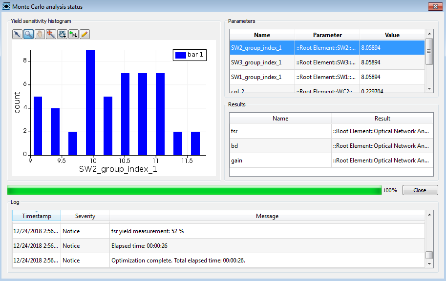
Close the "Monte Carlo analysis status" window and all the results will be shown in the Result View window.
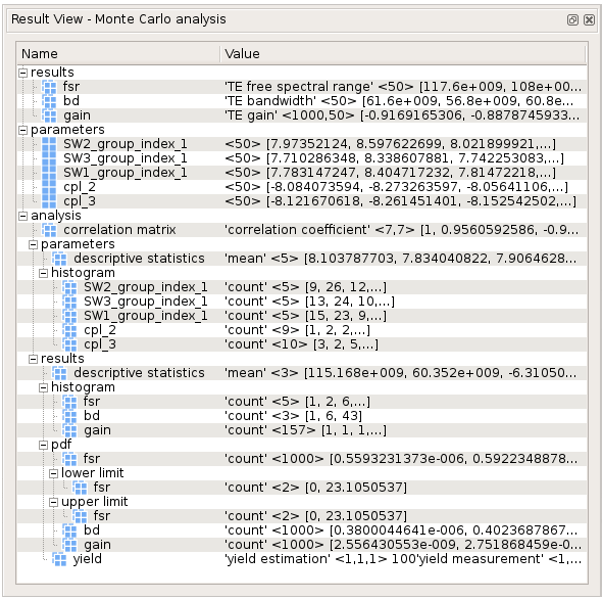
Viewing the results
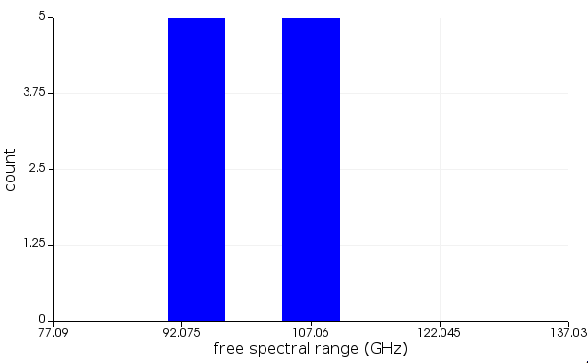
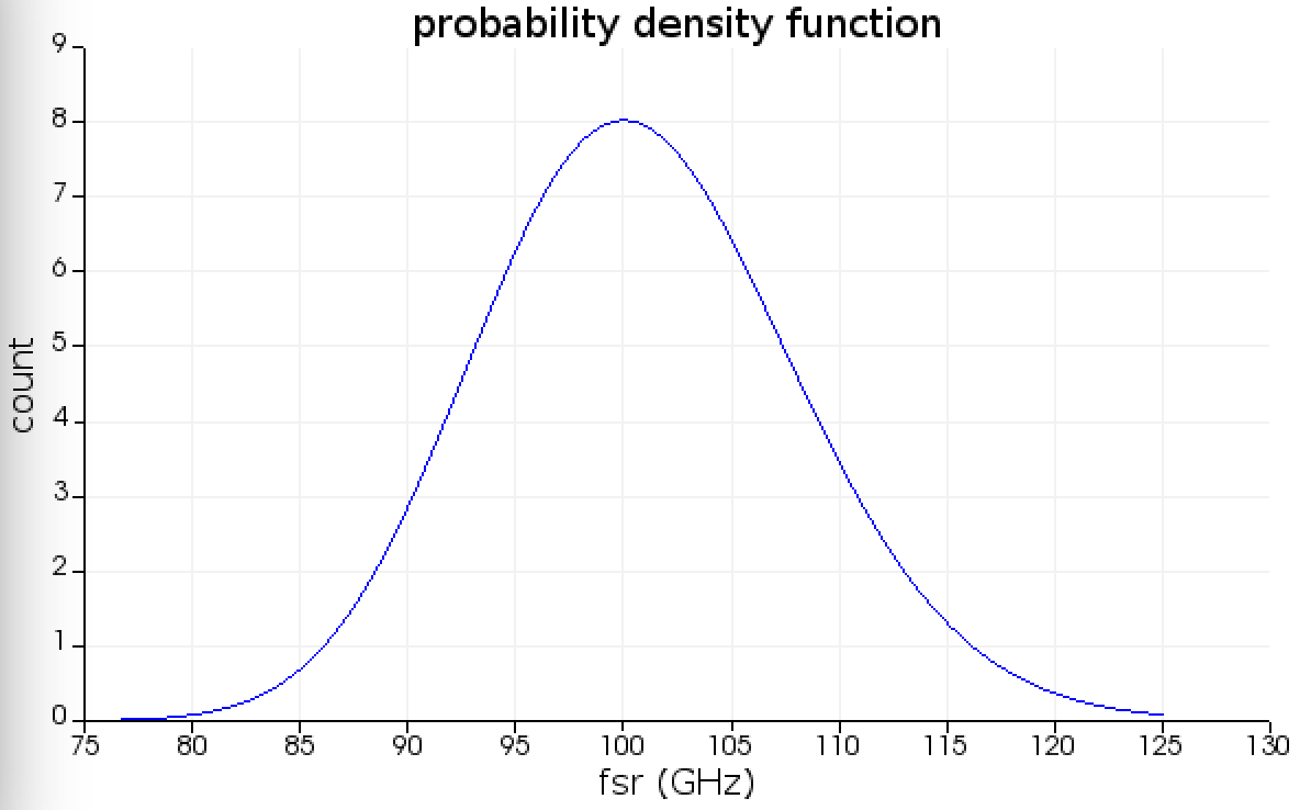
The Monte Carlo analysis results could also be plotted by using script commands. The commands below retrieve and plot the free spectral range histogram and probability density function.
# get & view Monte Carlo results
fsr = getsweepresult(MC_name, "analysis/results/histogram/fsr");
fsrCount = fsr.count;
fsr = fsr.fsr;

pdf = getsweepresult(MC_name, "analysis/results/pdf/fsr");
pdfCount = pdf.count;
pdfFsr = pdf.fsr;

histc(fsr/1e9, fsrCount, "free spectral range (GHz)", "count", "histogram");
legend("");
plot(pdfFsr/1e9, pdfCount, "fsr (GHz)", "count", "probability density function");
legend("");