Thermally tuned waveguide sensor

In this example, we will model thermal tuning of a waveguide sensor.  The waveguide sensor used in this example is a functionalized biosensor that senses the change in the effective index of the analyte using a Mach Zehnder configuration.  The same approach can be used to simulate chemical or other types of waveguide sensors.  The sensitivity of the sensor is calculated and is thermally tuned using a simple resistive heater.

Simulation set up

The device under investigation is a Mach Zehnder Interferometer (MZI) type biosensor with a functionalized surface.  The sensing arm (waveguide) is placed in a trench and a thin layer (30 nm) is created on its surface due to chemical reaction with the biomolecules (analyte).  The thin layer of analyte changes the effective index of the optical mode of the waveguide and affects the transmission of the MZI.  The fundamental TM mode of the 220 nm high and 800 nm wide silicon waveguide is used. The waveguide supports 3 guided modes: 2 TE-like modes and 1 TM-like mode.  A CW laser with a fixed wavelength of 1.55 micron is used as input to the MZI and an integrated photodetector is used at the output.  A resistive heater is used to tune the sensitivity of the biosensor.

Heat transport

Open the waveguide_sensor_heater.ldev file.  The waveguide sits on top of a 2 micron thick oxide layer on a silicon substrate.  A 5 micron wide and 5 micron deep trench is etched in the oxide surrounding the waveguide to create a channel for the analyte.  The analyte is treated as an insulator with a small thermal conductivity in the thermal simulation.  The resistive heater is a tungsten wire placed 2 micron above the waveguide and 2 micron away from the trench.  A uniform heat source is placed on the tungsten wire to model the heat generated in the heater.  The bottom of the substrate is kept at room temperature (300 K) using a fixed temperature boundary condition.  The top surface of the structure is assumed to have a convective boundary condition.  A 2D temperature monitor is placed in the vicinity of the waveguide to save the temperature profile to be exported to MODE.

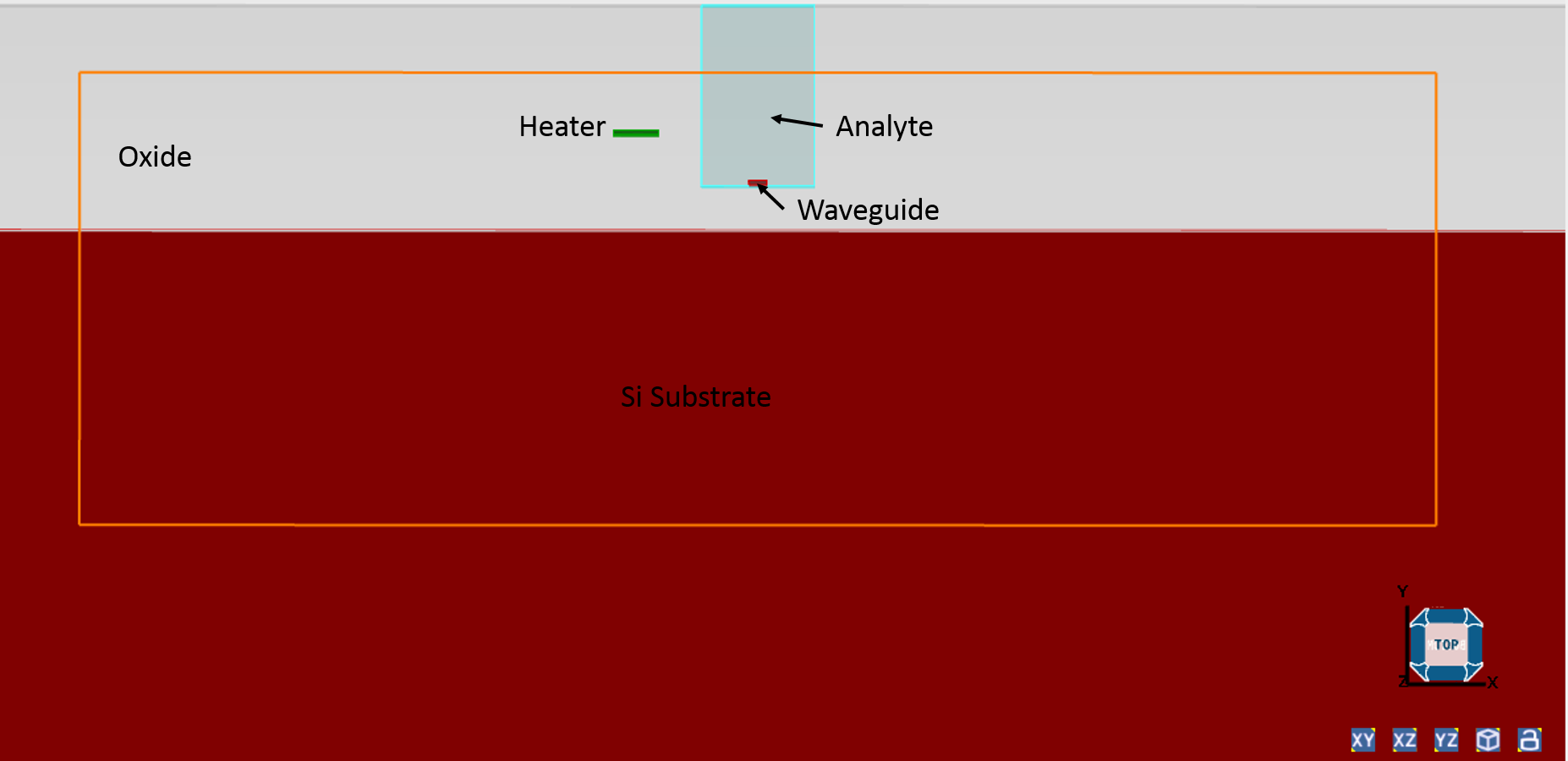
Figure 1

Optical response

Open the waveguide_sensor_heater.lms file.  The waveguide and the bottom oxide layers are created in MODE.  A 30 nm thin layer of analyte is placed on top of the waveguide.  The analyte is defined as a dielectric material and its index is set to 1.33.  Two "index perturbation" type materials are created based on silicon and silicon dioxide for the waveguide and the oxide layer.  The index perturbation material takes the index of the base material (silicon or silicon dioxide) and perturbs the index according to any imported temperature profile.  The temperature grid attribute is used to import the temperature profile from thermal simulation.

Figure 2

Circuit simulation

Open the waveguide_sensor_circuit_heater.icp file.  The top arm of the MZI consists on a passive waveguide and the bottom arm consists of a passive waveguide in series with two modulators.  The first modulator models the perturbation in the effective index for changes in analyte index.  The second modulator models the perturbation of the waveguide's effective index due to temperature variation caused by the heater.  The waveguide and modulator properties are imported from data saved from MODE simulations.  The optical network analyzer (ONA) is used to provide input to the MZI and to analyze the output.  

Simulation results

Thermal effect

Open the waveguide_sensor_heater.ldev file and run the simulation.  The thermal solver will solve for the heat transport in the device for an input power of 0.5 W per centimeter length of the waveguide (set by the norm length of the 2D solver).  Once the simulation is run, the 2D temperature monitor will contain the temperature profile of the waveguide and the bottom oxide.  Lock the mesh by right clicking on the HEAT solver object and save the file.  Next, perform a parameter sweep to change the heater input power from 0 to 1 W.  A paremeter sweep (Heat) has been included in the project file.  Running the sweep will change the power of the uniform heat source from 0 to 1 W in three steps and save the temperature profile from the 2D monitor.  Once the sweep has finished running, use the following scripts to save the temperature profiles in a .mat file to be exported into MODE.

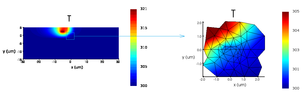
Figure 3

data = getsweepresult('Heat','T_profile');
matlabsave('temp_data.mat',data);

Next open the waveguide_sensor_heater.lms file.  The temperature data from the matlab file has already been loaded in the temperature grid attribute object.  Run the available parameter sweep to calculate the effective index of the TM mode for different heat input.  Once the sweep is run, you can visualize the result available in the sweep object.  Next run the script file get_dneff_vs_heat.lsf to calculate the change in effective index as a function of heat input at the heater and save it in a .txt file for Interconnect.  The script file also plots the change in effective index versus heater input.

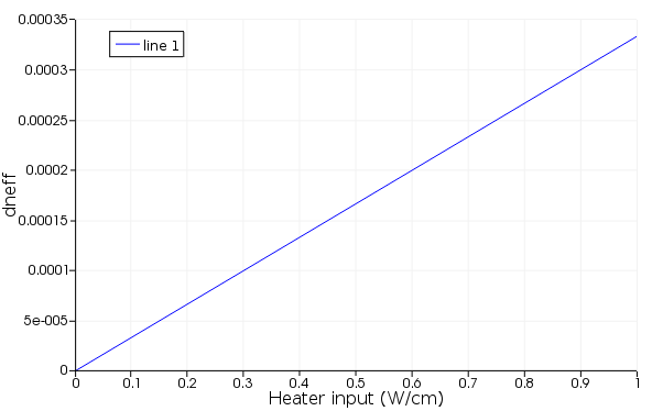
Figure 4

Biosensor sensitivity

Open the waveguide_sensor_circuit_heater.icp file.  The waveguide properties and the data for the modulator modeling the effect of analyte index is already loaded (make sure that the "mode_file_thermal_waveguide.ldf" data file is in the same folder as the project file).  The data for the modulator modeling index perturbation due to heater input can be loaded into the "T phase change" modulator.  To load the data, go to the property view window, enable "load from file" option, click on the "measurement filename" and select the text file saved from MODE simulation.  The amplitude is set to 0.5 which means a heater input of 0.5 W will be considered.  Run the simulation and view the transmission data from the ONA_1.  The FSR of the MZI is roughly 80 GHz.

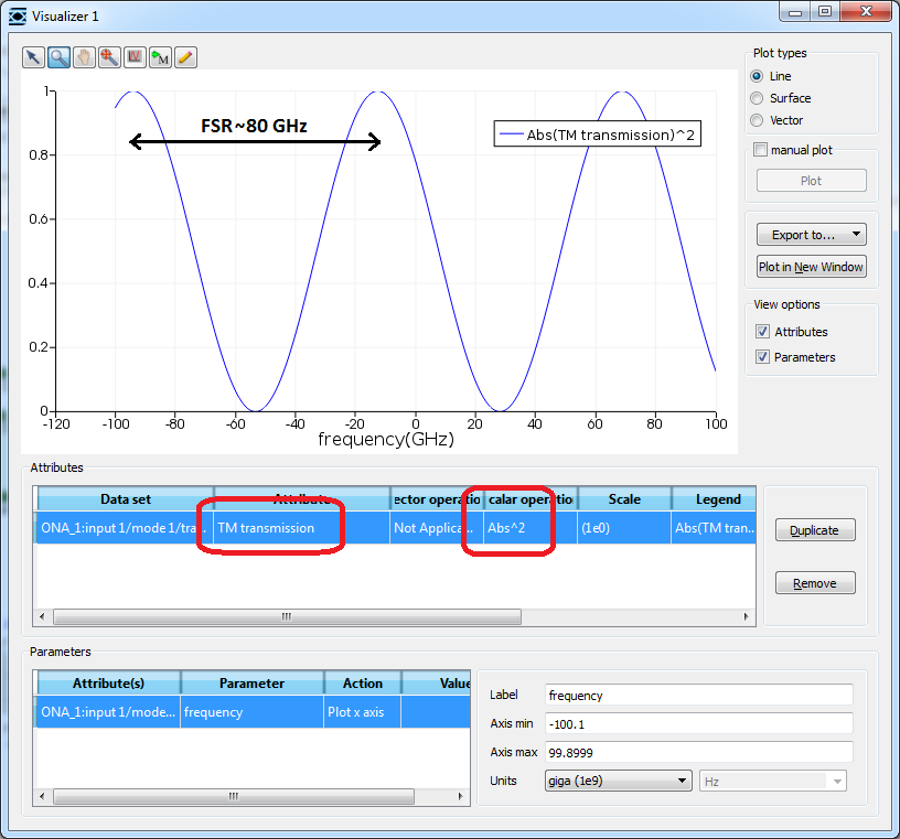
Figure 5

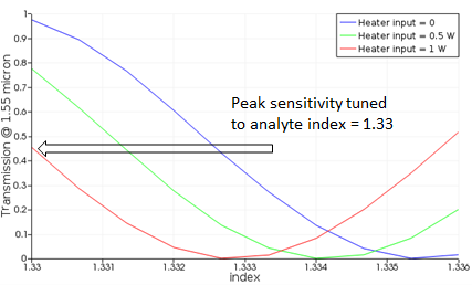
Next, run the nested sweep "sweep_Heat".  The sweep will calculate the transmission and peak transmission (transmission at center frequency) for different analyte index while varying the input power of the heater.  Once the sweep finishes running, visualize the result "peak".  The transmission of the MZI at center frequency (λ = 1..55 micron) will be plotted as a function of analyte index.  The biosensor is most sensitive at the analyte index where the slope of the curve is highest.  At zero input to the heater, the sensor is most sensitive for an analyte index of approximately 1.3325.  As the heat input power is increased, the index at which peak slope (sensitivity) is achieved lowers.  This information can be used to thermally tune the biosensor and make it most sensitive at the desired value of analyte index.

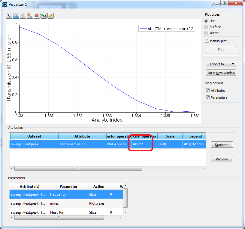
Figure 6

Figure 7

See Also

Index perturbation