This page explains how to simulate a light propagation in a tapered waveguide with 100μm length which delivers a light energy from a macroscopic region into a nano scale region. Two very similar simulations are constructed. The first uses a slightly different setup with a higher index substrate and a Gaussian beam source, and the varFDTD solver is used for this setup. The second simulation uses a homogenous cladding around the core and the fundamental mode of the waveguide is propagated using either the EME solver or the varFDTD solver. A comparison between the two methods and the advantages and disadvantages of each method are discussed.
Simulation setup
For the simulation file using the 2.5D varFDTD solver
In the tapered_waveguide_gaussian.lms simulation file, we consider an outlet tapered waveguide shown below. The substrate below the core is Al2O3, and there is air above the core. The width and the thickness of the input port are 4 μm and 2 μm, respectively and those of the output port are 0.4μm and 2 μm, respectively. A focused beam couples into the waveguide from the air region and the waveguide taper region is 100um in length. The simulation bandwidth is from 0.4 to 0.7 μm. The varFDTD solver in MODE will be used fore this simulation.

For the simulation file using both 2.5D varFDTD and EME solvers
In the tapered_waveguide_mode.lms simulation file, the same tapered core is used, but a uniform cladding of Al2O3 is used around the structure, and the fundamental mode of the waveguide is propagated rather than a Gaussian beam source. In the file, the EME solver region is active. The simulation can also be run using the varFDTD solver, and to enable to varFDTD solver and related monitors, simply right-click on the varFDTD solver in the Objects Tree and select the "Set as active" option from the right-click menu.
Results
For the simulation file using the 2.5D varFDTD solver
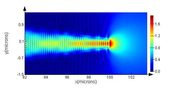
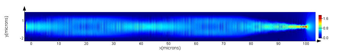
The figure below show electric field profile within the waveguide which is recorded on a profile monitor named "field_profile" for the tapered_waveguide_gaussian.lms simulation file.
For the simulation file using both 2.5D varFDTD and EME solvers
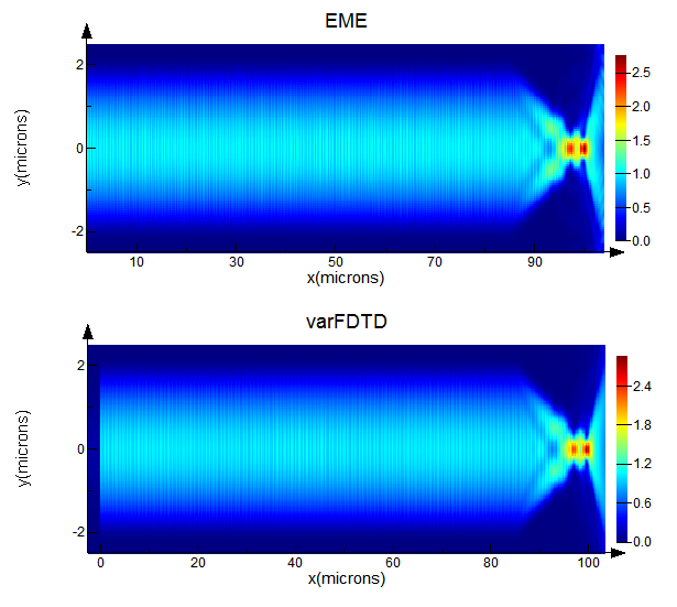
For the tapered_waveguide_mode.lms simulation file, below are the profile plots generated using the EME and varFDTD solvers.
The following shows the electric field amplitude through a slice of the structure at y=0 at around the output region of the taper showing that the results for both the EME and varFDTD method are close.

Discussion
Solver types
In the tapered_waveguide_gaussian.lms file, the varFDTD solver region is used rather than the EME solver region. There are a couple of reasons why the varFDTD method is preferable in this case.
- We want to simulate a broadband Gaussian beam source. Since the EME method is a frequency domain method, this would require re-running the simulation and solving for modes at each frequency point in the broadband range.
- We want to simulate the propagation of light in the air region beyond the taper output where there is a substrate. In the region after the output of the taper, the EME solver cross section would include air with the substrate below and no higher index core. In this case, the mode solver will predominately find modes that are confined in the substrate rather than finding the modes that propagate in the air region that overlap with the output fields from the taper. It would require setting up the EME solver to find a very large number of modes in the air region to get an accurate representation of the propagation in that region.
In the tapered_waveguide_mode.lms file, we can get similar results using the EME and varFDTD methods. A couple of reasons we may prefer using the EME solver for this simulation are:
- If we want to optimize the length of the waveguide or taper region. After the simulation is run once, we can get the results for different lengths of the structure without re-running the simulation by using the propagation sweep tool. See the Spot Size Converter getting started tutorial for an example of how the propagation sweep tool is used. Using the varFDTD solver would require running a simulation for each length.
- The EME solver gives results for multiple modes of interest with one simulation. In the EME solver ports we can specify multiple modes of interest for each input and output port and obtain the S-parameters of the device for all of the modes from a single simulation whereas the varFDTD solver would require injecting a different mode and running the simulation again for each mode.
Propagation in air
When using the EME solver object, the number of modes used to calculate the propagation in the air region beyond the taper is set to 100, which is relatively large compared to the number of modes needed to calculate the propagation in the waveguide region where the light is confined in the core. Since the light is diverging from the taper and traveling in different directions in the air region, we need many modes to represent the fields propagating there. For increased accuracy, the fields could be calculated just after the taper output and exported to FDTD where a far field projection can be done to simulate the propagation in air.
Related publication
- K. Takano, E. Jin, T. Maletzky, E. Schreck, and M. Dovek, "Optical Design Challenges of Thermally Assisted Magnetic Recording Heads," IEEE Trans. Magn., vol. 46, pp. 744–7507 (2010).