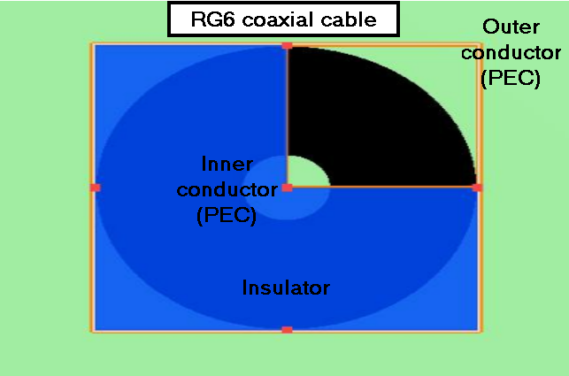
This topic describes a technique for calculating the impedance of a waveguide. The example structure is a standard RG6 coaxial cable.
To calculate impedance, we first calculate the voltage between conductors and the current flowing in the inner conductor. V is calculated by integrating the electric field along a path from the inner conductor to the outer conductor. I is calculated by integrating H around the inner conductor. Once V and I are known, it is trivial to calculate the impedance. We also calculate the cutoff frequency of this coaxial cable.
It is also possible to calculate the characteristic impedance using the built-in Power and Impedance Integration tool. For an example which uses this method, see Stripline.
Simulation setup
Cable dimensions
RG6 coaxial cable datasheets typically state following information:
|
Name |
Value in this example |
|
inner conductor radius (r) |
0.512 mm (18 AWG) |
|
propagation velocity (vc) |
0.85 c |
|
impedance (Z) |
75 ohm |
For the insulator, we use Semi-Solid PE with a relative permittivity of 1.29. Note that in the simulation setup, the background index is specified, not the background permittivity so we use a value of sqrt(1.29). The outer conductor radius can be calculated with the second formula below and we set the value to 2.23039 mm.
Coaxial cable standard formulas
$$Z=\sqrt{\frac{L}{C}}=\frac{1}{2 \pi} \sqrt{\frac{\mu_{0}}{\varepsilon_{0} \varepsilon_{r}}} \log \left(\frac{R}{r}\right) \approx \frac{138}{\sqrt{\varepsilon_{r}}} \log _{10}\left(\frac{R}{r}\right)$$
$$R=r e^{2 \pi Z} \sqrt{\frac{\varepsilon_{0} \varepsilon_{r}}{\mu_{0}}}$$
$$\varepsilon_{r}=\frac{1}{v_{c}^{2}}$$
$$f_{c}=\frac{c}{\pi(R+r) \sqrt{u_{r} \varepsilon_{r}}}$$
Conductor material definition
At GHz frequencies, most metals act like perfect electrical conductors (PEC) and we use the PEC material in the default material database. Note that we could use a material such as copper by creating a material with a high conductivity, and we would obtain similar results for most calculations. However, the penetration depth of the field into the copper is on the order of 10s of microns, so we would need to use a mesh size of smaller than 10 microns to accurately measure the loss.
Symmetry
The TEM mode of this waveguide is circularly symmetric. Therefore, we can use symmetric boundary conditions in the X and Y directions. Using symmetric boundary conditions will make the simulation faster.
Analysis
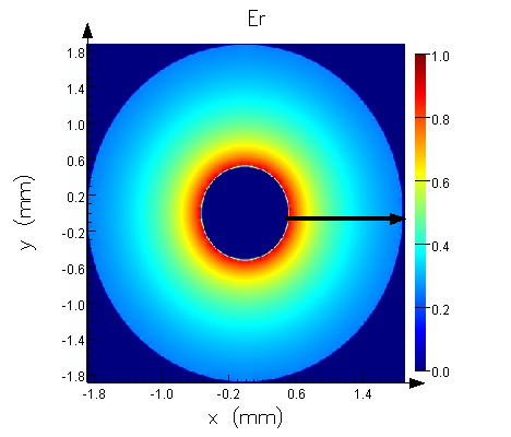
Impedance is defined as Z=V/I. The voltage can be calculated by integrating E between the two conductors. Similarly, the current can be calculated by integrating H around the inner conductor. These integrals are shown in the following figures.
Note that the following figures were created with a finer mesh than in the associated file. As a result, the E and H fields are smoother.
 |
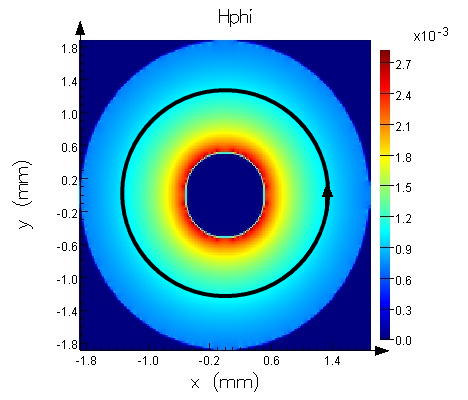 |
| $$V=\int_{r}^{R} E \cdot d r$$ | $$I=\int_{l o o p} H \cdot d S$$ |
Results
Impedance
After calculating the modes of this structure, run the analysis script. It will calculate the impedance by integrating the electric and magnetic fields, as described above. The theoretical impedance for this device is 75 ohms, the phase velocity is 0.85 c and the cutoff frequency is 29.5775 GHz. The script gives a calculated impedance of 75.9 ohms, a phase velocity of 0.88c and a cutoff frequency of 30.637 GHz.
Cutoff frequency
The fundamental TEM mode of a coaxial cable does not have a cutoff frequency, unlike all other modes. The TE mode has the lowest cutoff frequency. Below this frequency, the waveguide will be single mode. The theoretical cutoff frequency of the TE mode in this structure is 38GHz.
The cutoff frequency can be calculated with the following procedure:
- Set all boundary conditions to metal. Symmetry can not be used because the TE mode does not have the same symmetry as the fundamental TEM mode.
- Set the simulation frequency to 50 GHz and calculate the modes. The 2nd and 3rd modes will be the TE modes. These modes can be identified by their field profile (Ez is zero, but Hz is non-zero) and by the fact they have no loss at this frequency.
- Select the frequency sweep tab. Set the Stop frequency to 10 GHz. Select the 2nd mode and make sure that "track selected mode" is checked. Run the frequency sweep.
- The cutoff frequency is easiest to identify by looking at the effective index vs frequency and loss vs frequency. Below the cutoff frequency, the TE mode will have very high loss and an effective index of 0. Above the cutoff frequency, the TE mode will have a finite effective index and a loss of 0. A more accurate estimate could be found by reducing the frequency range around the cutoff point and repeating the calculation. Note that the plot created by the frequency sweep may show a positive or a negative loss - this occurs because the propagation direction (forwards or backwards) cannot be clearly defined when the effective index is 0. To create a plot showing only positive loss, select "Abs" under Scalar operation in the Visualizer.


