This topic compares analytical solutions and results simulated with the FDE solver for step-index and graded-index optical fibers.
Simulation setup
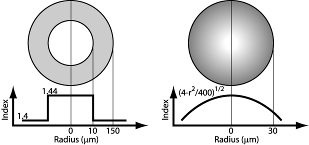
The figure above shows the step-index (left) and graded-index (right) fiber geometries and index profiles. The step-index fiber was tested at a wavelength of 1.55 µm, while the graded-index fiber was tested at a wavelength of 1 µm. The step-index fiber was created using two overlapping circle structures of silica (n=1.4) and a dielectric defined with index n=1.44. The graded-index fiber was created using a circle structure with index given by the equation sqrt(4*(1-(x^2+y^2)/40^2)).
Results
Analytical Solutions
The analytical solutions for the TM modes in the step-index fiber can be calculated using the MATLAB script step_index_fiber.m; alternatively, you can download the text file step_index_fiber.txt, which contains the calculated results.
In the graded-index fiber, the analytical solution for the effective index of the TE modes is given by the following expression:
$$N_{m n}=n_{0} \sqrt{1-\frac{\alpha}{h k_{0}}}$$
where
$${\alpha=2+2(m+n)}$$
$${k_{0}=2 \pi \frac{n_{0}}{\lambda}}$$
These analytical results will be used to validate the FDE calculations in the next section.
Step-index fiber
The script step_index_fiber.lsf calculates the effective indices of the TM01, TM02 and TM03 modes and plots the errors with respect to the analytical results, as a function of the number of grid points. The file step_index_fiber.ldf contains these modes previously calculated and saved in d-cards, which are imported by the script and used to identify the desired modes with the function bestoverlap.
The script also allows you to run the analytical calculation of the effective index and generate the error plot using Matlab. The flag "use_matlab" should be set to 1 to launch the Matlab calculations (Matlab Integration must be enabled).
The results below were calculated using "conformal variant 1" for the mesh refinement option (setting conformal_mesh_on=1 in the script). The accuracy of the results is reduced when conformal mesh is not used due to the effect of staircasing.
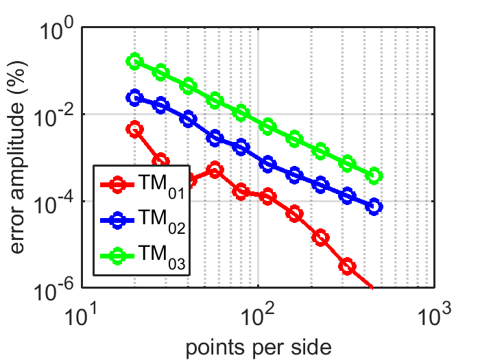

(Left) Magnitude of error of MODE calculation for TM modes of a step-index fiber, compared to analytic result at a wavelength of 1.55 µm. The x-axis denotes the number of grid points per side of the calculation region. (Right) The same figure generated using only built-in MODE functions (no Matlab interface).
Graded-index fiber
The script graded_index_fiber.lsf calculates the effective indices of the TE01 and TE11 modes and plots the corresponding errors with respect to the analytical results, as a function of the number of grid points. The file graded_index_fiber.ldf contains these modes previously calculated and saved in d-cards, which are imported by the script and used to identify the desired modes with the function bestoverlap. The script also explores the dispersion properties and associated errors of the TE01 mode.
As before, you can generate the dispersion and error plots using Matlab. The flag "use_matlab" should be set to 1 to launch the Matlab calculations (Matlab Integration must be enabled).
In this case, the conformal mesh does not have a significant impact on the accuracy of the results because the index changes smoothly in the fiber, as opposed to the sudden changes in the step-index fiber. The results below were calculated using the "conformal variant 1" option.


(Left) Magnitude of error of MODE calculation for TE modes of a graded-index fiber, compared to analytic result at an operating wavelength of 1 µm. The x-axis is the number of grid points per side of the calculation region. (Right)The same figure generated using only built-in MODE functions (no Matlab interface).


(Left) Dispersion of TE01 mode in graded-index fiber calculated by MODE (o) compared to the analytic solution (solid line). 80 grid points per side were used in this calculation. (Right) The same figure generated using only built-in MODE functions (no Matlab interface).


(Left) Magnitude of error of MODE calculation for dispersion of TE01 mode of a graded-index fiber, compared to analytic result. 80 grid points per side were used in this calculation. (Right) The same figure generated using only built-in MODE functions (no Matlab interface).
|
Note: Effect of detailed dispersion setting on the accuracy of the dispersion The detailed dispersion option was disabled in the frequency sweep to calculate the dispersion of the TE01 mode in the graded-index fiber. In this case the frequency sampling is fine enough to get accurate results for the dispersion. In fact, enabling the detailed dispersion with the default fractional wavelength offset (0.0001) will lead to larger errors in the dispersion. The reason is that the effective index changes very little in the wavelength range 1-1.5um, as shown below
Therefore, if the frequency step used to calculate the derivatives of the effective index is too small, the change in the effective index can become comparable to the accuracy of the effective index calculation, leading to numerical errors in the derivatives. |
