
This example shows how to calculate the Nonreciprocal Phase Shift (NRPS) of some nonreciprocal Magneto-Optical (MO) devices for integrated optics.
Background
The NRPS is a widely used phenomenon to describe the nonreciprocal effects of an MO device, where its basis is Faraday rotation. If the medium of the MO device is magnetized in the transverse direction (eg, z), the anisotropic permittivity can be written as, for forward and backward propagation fields,
$$ \varepsilon_{\text {forward}}=\left(\begin{array}{ccc}{\varepsilon_{x x}} & {i \varepsilon_{x y}} & {0} \\ {-i \varepsilon_{x y}} & {\varepsilon_{y y}} & {0} \\ {0} & {0} & {\varepsilon_{z z}}\end{array}\right) $$
$$ \varepsilon_{\text {backward}}=\left(\begin{array}{ccc}{\varepsilon_{x x}} & {-i \varepsilon_{x y}} & {0} \\ {i \varepsilon_{x y}} & {\varepsilon_{y y}} & {0} \\ {0} & {0} & {\varepsilon_{z z}}\end{array}\right) $$
where the wave is TE polarized (Hz strongest) traveling along the x axis. In this case, the propagation mode will experience some Faraday rotation effect on the xy plane. Due to the perturbation, the forward and backward propagating waves will then have a slightly different propagation constant. The difference in the propagation constants is the NRPS:
$$ N R P S=\beta_{\text {forward }}-\beta_{\text {backward }} $$
where beta_forward and beta_backward are the propagation constants of the forward and backward propagation waves respectively. Phase shift can therefore be achieved and make it possible for applications such as optical isolation in integrated optics.
Conformal meshing for the grid attribute should be disabled for MO calculations. This avoids significant errors in the mesh cells at the interface between the MO material and the surrounding materials. For more information, please refer to the gird attribute tips page.
Simulation with FDE solver
Since release 2020a R7, the FDE solver in MODE can handle MO simulations. The simplest analysis of waveguides directly solves for the effective indices (and group indices) of MO waveguides. The file [[MO_NRPS_Balhmann_FDE.lms]] contains the structure defined in [1]. There are 3 designs, A, B, and C which can be set in the "::model" group, as well as the rib height, rib thickness, and total thickness. The "x max" boundary condition uses PML to eliminate the slab modes which can cause challenges tracking the desired guided TM mode.
Referring to [1], the anisotropic permittivity tensors can be written as,
$$ \varepsilon_{\text {forward}}=\left(\begin{array}{ccc}{\varepsilon_{\mathrm{xx}}} & {0} & {0} \\ {0} & {\varepsilon_{\mathrm{yy}}} & {i \frac{2 n \theta_{F}}{k_{0}}} \\ {0} & {-i \frac{2 n \theta_{F}}{k_{0}}} & {\varepsilon_{z z}}\end{array}\right) $$
$$ \varepsilon_{\text {backward }}=\left(\begin{array}{ccc}{\varepsilon_{\mathrm{xx}}} & {0} & {0} \\ {0} & {\varepsilon_{\mathrm{yy}}} & {-i \frac{2 n \theta_{F}}{k_{0}}} \\ {0} & {i \frac{2 n \theta_{F}}{k_{0}}} & {\varepsilon_{z z}}\end{array}\right) $$
where ΘF is the Faraday rotation angle, k0 is the vacuum wave number, n is the isotropic refractive index.
In this case, the waveguide has a uniform cross-section on the xy plane where the mode propagation direction is z. The mode has the strongest field components in the y-direction - TM mode. Magnetization is applied along the x-direction. The mode will experience some Faraday rotation effect on the yz plane. Therefore, it is okay to apply symmetry along the y-axis.
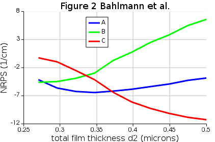
The script file [[MO_NRPS_Bahlmann_calculation_FDE.lsf]] can be used to calculate the NRPS for all 3 designs. This script also calls [[MO_NRPS_Bahlman_material.lsf]] to update the material properties due to the reversal of the magnetic field.
The script produces the following figure:

which accurately reproduces the results shown in fig. 2 of [1]. The noise observed at certain thicknesses is due to coupling with slab waveguide modes which can be eliminated by increasing the simulation region area. The "x max" boundary can also be set to Metal rather than PML, but more care must be taken with mode tracking through the sweep.
Simple direct simulation in FDTD
In this simple approach, two simulations will be run with waves injected in opposite directions near the +x and -x simulation boundary. The phase accumulated by the forward and backward propagating wave is recorded by an x linear frequency monitor, and being subtracted according to the above equation. By plotting the phase difference against the propagation distance, NRPS can be calculated by finding the slope of the plot. This method is not efficient for the study of the NRPS of straight waveguides but it shows how the simulations can be run in FDTD for more complex geometries.
Simulation setup
In this example [2], we set εxy = 0.005. The isotropic refractive indices of Si and Ce:YIG are 3.477 and 2.22. Discussed in the Matrix transformation page, the anisotropic tensor is diagonalized and transformed by the grid attribute. Below is the top view of the device with a TE mode injected along the x-axis.
| [[Note]]: This simulation is set up on the xy plane whereas the publication has the structure set up on the xz plane. |

Open [[MO_NRPS_Zhou.fsp]] and run [[MO_NRPS_Zhou_material.lsf]]. The script file shows how eps_forward and eps_backward are diagonalized and the grid attributes are set up. The [[MO_NRPS_Zhou_calculation.lsf]] will then run two simulations for each configuration to obtain the propagation constants for the forward and backward propagating waves.
Results
Since the forward and backward propagating waves have a different propagation constant, therefore the phase accumulated is going to be different. By subtracting the phase of the waves, the phase difference can be calculated. The fit command is used to find the slope of the phase difference and therefore the NRPS.

Repeat the process for different silicon thickness and script file can generate a plot shown below for MO(+)/Si/MO(-) and MO/Si/air configuration, corresponding the figure 2 in ref. [1]. Disable the MO_neg rectangle to run the simulation for MO/Si/Air configuration.

Bandstructure approach in FDTD
The other way to find the NRPS is to make use of the group velocity definition,
$$ \Delta \beta=\frac{\Delta \omega}{V_{g}}=\frac{\omega_{\text {forward }}-\omega_{\text {backward }}}{c} n_{g} $$
where Vg and ng are the group velocity and group index. The bandstructure approach is not efficient compared to using the FDE solver but it can be extended to study structures with periodic patterning, such as sub-wavelength grating waveguides. This approach employs the Bloch boundary conditions to mimic an infinitely long waveguide. Since here we study a waveguide that is not actually periodic, we can use a single mesh cell in the direction of propagation. The bandstructure analysis group is used to find the frequency of the mode supported by the Bloch vector. Due to the perturbation from the magnetization, the forward and backward propagating waves will have a different propagation constant. Here we use the bandstructure approach to reproduce the results of Figure 2 of [1], to compare with the FDE solver results above.
Simulation setup
Discussed in the Matrix transformation page, the anisotropic tensor is diagonalized, and transformed by the grid attribute. By switching the sign in the Faraday rotation coefficient, the bandstructure analysis group is able to return the resonance frequencies due to the presence of the perturbation. Symmetric boundary conditions on the y axis can be applied to this simulation because the rotation is only effective on the yz plane, therefore, the time monitors are only present in the +x simulation region. The image below shows the xy pan view of the device with the TM mode being injected along the z-axis.

The group indices are calculated by the FDE solver, open [[MO_NRPS_Bahlmann_group_index.lms]] and run the [[MO_NRPS_Bahlmann_group_index.lsf]]. Run the FDE simulations to generate a .mat that is used to carry the group indices for the NRPS calculation in FDTD. The design parameters for the FDE simulations are set in the script file, make sure the same parameters are set in the FDTD simulations. Open [[MO_NRPS_Bahlmann.fsp]] and run [[MO_NRPS_Bahlmann_calculation.lsf]], the script file will automatically run two simulations by switching the sign of the Faraday rotation angle by calling [[MO_NRPS_Bahlmann_material.lsf]]. The phase calculation script will then extract the resonance frequencies recorded by the bandstructure analysis group to calculate NRPS according to the group velocity equation above.
Results
Run the [[MO_NRPS_Bahlmann_calculation.lsf]], it will run two simulations (backward and forward). The bandstructure analysis group can return the spectrum for both simulations. Once the simulations are done, enter the command below to generate a plot for the spectra.
plotxy(f_for*1e-12, spectrum_for, f_back*1e-12, spectrum_back);

The spectra are slightly offset due to the magnetic perturbation. We can then use the find command to find the peak frequencies. Alongside with the group indices returned by the FDE solver, the NRPS can then be calculated. To obtain some initial results, the simulation time in FDTD is set to 100 fs. Users should use a longer simulation time to better distinguish the peak positions and therefore more accurate NRPS. Note the spectrum returned by the bandstructure analysis has 500000 points to make sure the point at the peak is resolved.
Now change the commenting in MO_NRPS_Bahlmann_group_index.lsf to set design={"A","B","C"}; instead of just design={"A"};, and d2=linspace(0.27e-6,0.5e-6,10); instead of a single value for d2. Rerun this script to recalculate the group indices.
Then, change the commenting in MO_NRPS_Bahlmann_calculation.lsf to use the same values of design and d2. Rerun the script and the following plot will be generated.
Here, we have reduced the range of d2 to reduce the number of simulations, but the agreement with the FDE results and with [1] is good.
Convergence
To obtain more reliable and accurate results, convergence testings is required:
- x and y span: In some situations (d2 < 0.3 um), the mode might have a longer tail where it will require larger source and simulation span to include the long tail.
- Simulation time: The waveguide in the simulation is supposed to be infinitely long, a longer the simulation time will allow the bandstructure analysis group to collect more data to return a more accurate f_peak.
- Mesh size: Finer mesh may be required to resolve the mode profile in order to better simulate the Faraday rotation effect.
- Bandstructure analysis group: There are only a limited number of time monitors used in the bandstructure analysis group. The position and number of time monitors can affect the results slightly, this should be also considered in convergence testing. Ideally, the monitors should be placed at the strongest field locations.
Related publications
- N. Bahlmann et al, "Improved Design of Magnetooptic Rib Waveguides for Optical Isolators", Journal of lighware technology, 1998.
- H. Zhou et al, "Analytical calculation of nonreciprocal phase shifts and comparison analysis of enhanced magneto-optical waveguides on SOI platform", Optics express, 2012