3D OLED with hexagonal lattice symmetry

This section shows how a 3D multi-layer OLED structure with hexagonal PC patterning can be simulated efficiently with FDTD. In this hexagonal OLED example, two simulation approaches are discussed: 1) using a parameter sweep to sweep the over the distributed dipole locations in the entire hexagonal unit cell. 2) using an unfolding method to make use of the hexagonal lattice symmetry.

OLED_3D_hex.fsp

Hexagonal symmetry

As with square lattice, we can symmetry to approach an OLED with hexagonal PC symmetry, to reduce the total number of simulations from 48 to 6. The steps are outlined below:

Step 1:

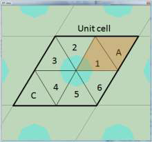
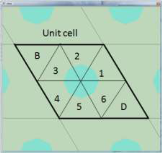
In the case of a hexagonal lattice, the unit cell is given by a parallelogram. In order to understand how to apply symmetry, we divide the unit cell into 8 triangular regions as shown below:

Step 2:

Using the fact that the lattice has 60 degree rotational symmetry, this can be reduced to regions A and 1 (shaded regions above).

Step 3:

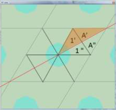
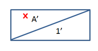
We further recognize the symmetry along the 30 degree line, and further reduce regions A and 1 to A' and 1'. This means that the result of a dipole place in an arbitrary location in 1'' can be determined from the results for a dipole in the same relative position in 1'.

Step 4:

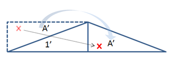
Using the results from steps 2 and 3, this means that the result of a dipole at position X in 1' can be used to determine the result of a dipole in the positions "O":

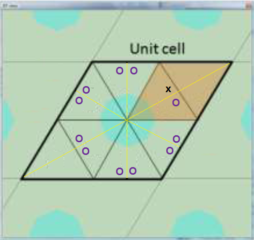
And the result of a dipole at position X in A' can be used to determine the result of a dipole in the positions "O":

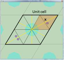
We have, therefore, reduced the number of dipole locations from 16 to 2, which means that we have reduced the total number of simulations from 48 to 6.

Step 5 (optional):

Here, we must recognize that the unit cell may also be given by a parallelogram shown below

In order to take the 2 types of unit cells into account, one can average the far-fields from these 2 unit cells. No extra simulations are required to do this since the results for one type of unit cell can be completely determined by the results from the other. However, if enough points are simulated within one orientation of the unit cell, this step over averaging over different orientations is not necessary and may not improve the results.

Note: even though we were able to reduce the number of simulations significantly, it is likely that 2 dipole locations (in 1'+A') will not be enough for an accurate simulation, and one should run a convergence test to make sure of this.

Simulation setup

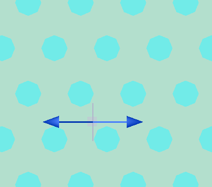
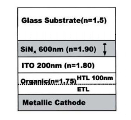
Again we consider a structure similar to the one propose by Chutinan et al, letting all materials, except the cathode, be loss less dielectrics. Starting with a simulation span of only 8x8 \(\mu\)m²  in the x and y plane, the simulation file OLED_3D_hex.fsp contains a parametrized OLED structure. Please note that all the children of this structure are fully deleted each time a parameter is changed, so you should not add or remove objects from this group.

Using a parameter sweep (no unfolding method applied)

In this approach, we will try to assign multiple dipoles to the entire unit cell. The reason to pick these dipole locations (instead of simple uniform 4x4 distribution) is to make it easier to understand and compare it with the folding method discussed in the following section. Parameter sweep is employed to run multiple simulations for each dipole location. In the figures shown below, the unit cell is divided into several regions, i.e., 1, 2, ... ,6 and A, C. The "x" and "o" indicate the dipole locations (without the unfolding method, we will run simulations with all dipole locations). In the file OLED_3D_hex.fsp, it sweeps over the dipole locations in the 1, 2, ... ,6 and A, C regions. In each region, there are two dipole locations. At each dipole location, three simulations are run - each with an x, y and z polarized dipole source resulting in 48 (8x2x3) simulations.

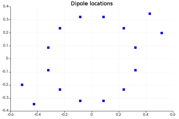
Dipole locations for parameter sweep

The dipole locations are generated based on the following script: The first twelve points in region 1 to 6 are generated based on a radius from the center of the PC. The following four points are then spatially transformed, i.e., 1', 1'' to C', C'' and 4', 4'' to A', A'' respectively. This allows dipoles to distribute to the entire unit cell. The xr and yr are not the actual positions, but the parameters normalized to the period of the PC lattice. The last line of this script can generate a plot that shows all sixteen dipole locations.

xr=matrix(16); # x positions of the dipoles
yr=matrix(16); # y positions of the dipoles
p= getnamed("OLED structure","pc period"); # period of PC
theta=linspace(15,345,12); # representing region 1', 1'', 2',...,6''
xr(1:12) = 0.15e-6*cos(theta*pi/180)/p; # forming a circular distribution
yr(1:12) = 0.15e-6*sin(theta*pi/180)/p;
xr(13:14)=xr(1:2)-3/4; # transform from region 1', 1'' to C', C'' in x-direction
yr(13:14)=yr(1:2)-sqrt(3)/4; # y-direction
xr(15:16)=xr(7:8)+3/4; # transform from region 4', 4'' to A', A'' in x-direction
yr(15:16)=yr(7:8)+sqrt(3)/4; # y-direction
plot(xr,yr,"","","Dipole locations","plot type = point"); # the parametrized dipole locations

The extraction efficiency enhancement and angular distribution plots

The plots below are the results generated by OLED_3D_farfield.lsf. Users will have to change "project_in_air" to "1" or "0" in the script file in order to view the enhancement in air or glass. The results are averaged by the "mean" option in the parameter sweep. Note that the results are sensitive to the dipole locations. Testing convergence is encouraged, for example, changing the dipole distribution would noticeably change the pattern of the plot. This behavior should converge when there are more number of dipoles distributed in the unit cell. Moreover, some hotspots may be observed in the far field plots. This could be due to not enough dipole locations. In addition, region B, D and etc can also be added to the sweep, if needed. Users can modify the above script to change the dipole locations.

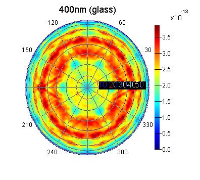
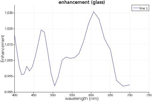
OLED_3Dhex_sweep_farfield_glass                                OLED_3Dhex_sweep_enhancement_glass

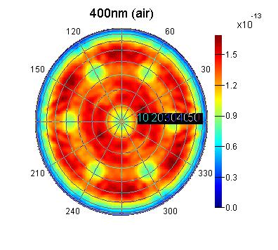
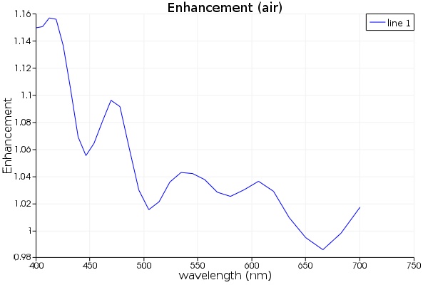
OLED_3Dhex_sweep_farfield_air                                     OLED_3Dhex_sweep_enhancement_air

Using the hexagonal symmetry unfolding method

Users are strongly encouraged to look at the above method (using the parameter sweep), before employing this advanced method.

In this approach, we are taking the advantage of the hexagonal lattice symmetry. Instead of running simulations at all dipole locations in the above section, only dipole locations in a particular region are run to reduce the number of simulation needed. Then the results are unfolded using the lattice symmetry. The unfolding process is a post-processing carried out via Lumerical's powerful scripting environment. We can use region 1' and A' to represent the entire unit cell due to the given lattice symmetry. Therefore, we only need to set up dipoles in these two regions. Each time the script is run, a dipole location is chosen based on a random number. The dipole can fall into either region 1' or A'. Then the results are unfolded, from 1' to 1'', 2', 2''...6'', and from A' to A'', C', C'', accordingly. If you would like to have more accurate results, you can set up more dipole locations in these two regions. The setup instructions below allow you to have as many dipole locations as you want, in a random distribution.

We will start with the same simulation setup using the same fsp file. To make use of this lattice symmetry, we will follow a modified process using script to "sweep" through the randomly picked dipole locations.

Seeding Dipoles

1. Open the file OLED_3D_hex.fsp and verify that the parallel settings are correct for your computer system.
2. The script file OLED_3D_hex_simulations.lsf is based on the description above. In the User Input, users can choose the total number of dipole locations, and the random seed. A different random seed with a low number of dipole location (

A random position in a rectangle (sqrt(3)/4 by 1/4) is generated using a random function.

If it is positioned in the upper triangle, the position is moved as below. If not, leave as is.

Rotate the point by 30 degree using rotation matrix. This position will determine either this dipole location is in region 1' or A'. And then generate three fsp files (polarization x, y and z) for this location, and pass the simulations to the job manager to run

Symmetry unfolding operations

1.  After all the jobs are completed, run the script file OLED_3D_hex_analysis.lsf. This file will load all the individual simulations and calculate the angular distribution of the light in either the substrate (glass) or the air (refer to the far_field_change_index analysis group). This script uses the results of the small number of simulations and, through symmetry unfolding operations, reconstructs the angular distribution from the incoherent superposition of all the dipole locations in the unit cell. This advanced process can take up to several hours depending on the size of the simulation used. Users can reduce the angular resolution to speed up the script initially, but will need reasonable resolution to generate the plots below.
2. Once the calculations for the angular distributions are complete, the script will generate a figure plotting the extraction efficiency enhancement and angular distributions. The analysis script will also save the unfolded data to a .ldf file.

Results and Discussion

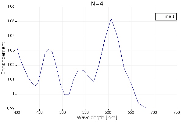
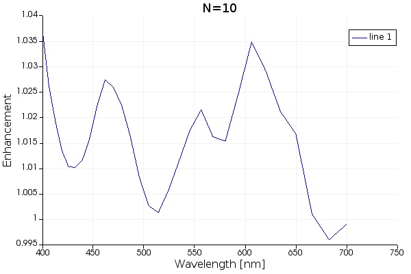
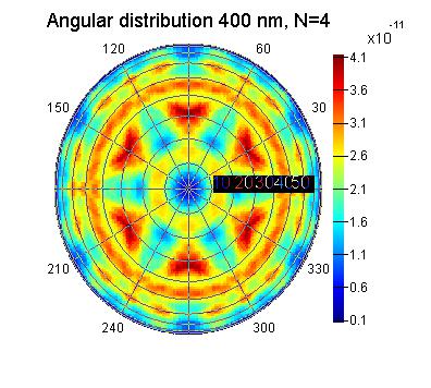
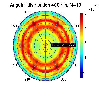
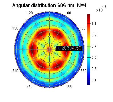
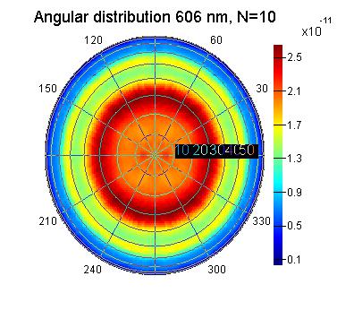
The figures below show some properties of the enhancement of the extraction efficiency and far field pattern with different number of dipole locations distributed in regions 1’ and A’. More number of dipoles should in principal lead to more converged results. Note the color bar scale changes because the far field plots are summed while unfolding.

As the case for the rectangular lattice, only a modest enhancement can be seen here for the hexagonal PC lattice, but could be improved with some design modifications.

Enhancement

See also

Far field change index analysis group