In this example, FDTD is used to simulate a coaxial-fed quarter-wavelength monopole antenna mounted over an infinite metallic ground plane. First we get the resonant frequency, then we analyze the antenna’s return loss, directivity, and far-field patterns with the help of the directivity analysis group. Because PEC is involved, exceptionally-finer mesh is used at the feed to accurately describe mode source and thus the inject power.
|
Note : Directivity analysis group As an instructive starting point, the Directivity analysis group page shows how to calculate the directivity of a simpler dipole source radiating over an infinite ground plane. |

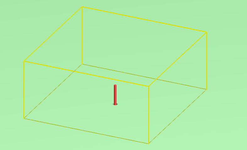
The quarter-wavelength monopole mounted above a ground plane and fed by a coaxial waveguide is a popular antenna used in wireless mobile communication systems. An illustration of the monopole is shown in the figure. In some instances, it is useful to consider the ground plane as an infinite perfect electrical conductor (PEC) boundary. The induced currents onto the ground plane contribute to the total radiation. Using image theory, it can be shown that the ground plane introduces a λ/4 image and system can be replaced by an equivalent λ/2 dipole. The directivity analysis group employs image theory to determine the farfields of an antenna situated over an infinite ground plane. It should be emphasized that the equivalent dipole gives the correct fields for the antenna system only above the ground plane (z>0, 0≤θ≤π/2). More details can be found in the Directivity analysis group page. The monopole antenna is designed to be a quarter wavelength at its resonance frequency, at which it is well matched, radiates efficiently, and possesses the typical donut shaped pattern seen for an electric dipole. However, the presence of the ground plane will redirect radiation away from the ground plane, resulting in higher directivity.
Simulation Setup
In this example, the monopole antenna is constructed from a vacuum-filled coaxial waveguide whose outer conductor is shorted to an infinite ground plane and whose inner conductor extends above the ground plane by a height λ0/4 where λ0=125mm (f0 is around 2.4 GHz). The inner and outer conductor radius of a=1.17 mm and b=2.20 mm was chosen to give a theoretical characteristic impedance of 37.5 Ω. The coaxial waveguide extends out the bottom (z min) FDTD boundary. Since this example is at microwave frequencies, the metals are approximated as a PEC. The ground plane is modeled using a ring which extends outside of the simulation region, rendering it infinite. Special override mesh regions are applied in "Mesh Group" in order to obtain accurate result.
|
Note : Mesh order and feed line through ground plane Whereas a ring is used for convenience here, in some application a solid 3D or 2D rectangle is more appropriate, which does not have an open interior to pass an antenna feed through. These requires careful attention to the mesh order of the coaxial feed and the ground plane to ensure the feed is properly simulated. |
The Directivity analysis group is used to set up the monitors and find the directivity of the monopole antenna. The x, y, and z span of the monitors are set to be in a uniform mesh by "directivity box",which should not be close to PML. In addition, setting the distance between the antenna and monitors to be about λ0/4 is good practice to have accurate monitor result. As long as the power in the near field is accurate, the power in the far field calculation should be accurate. Convergence testing of the group span (by trying a larger span and ensuring that the results don’t change) is recommended. The down sample variable is set to 1, so that no down sampling occurs on the monitors. To reduce simulation memory, do not use uniform mesh in the whole simulation region, instead, use override regions.
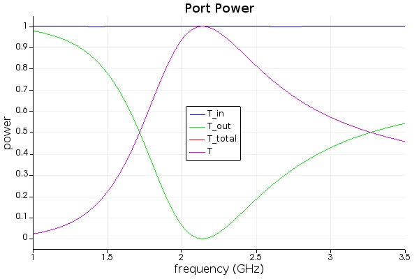
A Port is placed near the bottom edge of the simulation region to inject and measure the coaxial TEM mode over a frequency range of 1.0GHz to 3.5GHz. See the Port Group page for more details on setting up the Port. A frequency resolution of 301 points across the band is defined in the global monitor settings, which is not the normal setting.
|
Note : Placement of the source The source should be placed at least λ0/4 away from any discontinuities (such as the PEC ground plane) to obtain accurate results. Since the monopole region uses much finer mesh, the port is located about λ0/2 away. |
A mesh accuracy of 6 (unusually high) is used for the simulation region, and two override regions are used to ensure that the near fields are sampled to a high enough resolution to give accurate far field results. To resolve the cross-section of the coaxial line, the PEC interface, and the length of the monopole antenna, mesh override region is placed over the coax and monopole.
|
Note : Mesh Size on Ground Plane Interface The results from the far field projection calculations can be sensitive to the mesh around the interface of the PEC ground plane. It is recommended to use a fine mesh at the interface. We use a much finer mesh "coax feed" in the central region where field changes quickly, whereas use mesh accuracy 6 for the rest region. |
|
Note : Mesh Size on Monitors While λ0/10 is a good starting point in most examples for setting the mesh size on the monitors, in this example the mesh size is roughly λ0/40 (at the highest frequency) in an effort to obtain very accurate results. |
PML boundaries are specified on all boundaries to be at least λ0/4 thick to minimize PML reflections. These reflections would skew the far-field results of the monitors. To speed up the simulation, symmetry boundaries are specified on the x min and y min boundaries.
|
Note : PML Thickness While λ0/4 PML thickness is a generally adequate, the effect of PML thickness should be tested. In cases where the mesh size is very fine in the directions transverse to the PML's surface but coarsely meshed normal to the PML's surface (i.e., a high aspect ratio mesh grid of 10:1 or more), the PML may need a thickness of up to λ0. |
|
Note : Advanced Option - Snap PEC to yee cell boundary When the "snap pec to yee cell boundary" option is enabled in the FDTD object's advanced option tab, the interface of any PEC is forced to align with the Yee cell boundary (more details can be found in Simulation - FDTD). It is recommended that for RF applications this option always be turned on in antenna applications so as to improve the calculation of radiation efficiency, as well as match FDE's meshing. |
In many simulations, higher mesh accuracy like in this example is usually not necessary. However in this example, since the results are very sensitive to the mode source and the monitor box, exceptionally-finer mesh has been used. Users are encouraged to do some converging tests, in particular the source power and the near field power recorded by the monitors.
Results and Analysis
Powers and Reflection
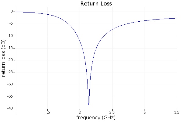
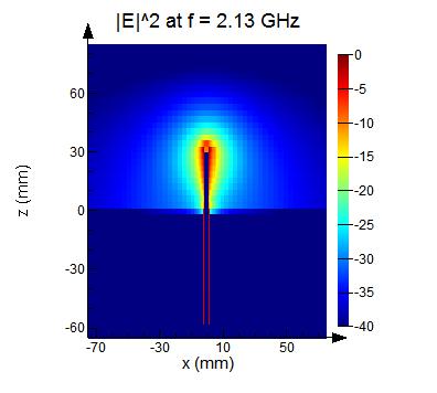
After running the simulation, the Monopole_Antenna.lsf script is used to generate the monopole antenna’s performance and radiation properties. This script first finds the reflection seen from Port 1 (S11) of the coaxial line (return loss =-20log10|S11|) as shown in the figure on the left. From the frequency response of S11, the script determines the resonant frequency (f=2.133GHz) from the smallest value of S11 (-38dB). This resonance frequency is about 10% of the designated resonance of 2.4GHz, in which the difference is attributed to fringing fields on the end of the monopole making its effective length greater than its physical length. Furthermore, the theory does not account for the impedance mismatch introduced by the feed’s discontinuity at z=0. The electric field intensity at the resonance is shown in the above figure on the right.
|
Note : Power Conservation Users should check that the total power going through the directivity monitor box is the same as the power going through feed to the desired accuracy. This ensures that the computed radiation results are accurate. For example, if you need your radiation efficiency to be accurate to plus or minus 0.5%, then power conservation in the near field must hold to within 0.5%. If this is not the case, the far field results (which include the radiation efficiency) will be less accurate. |
The directivity analysis group is then used to calculate the far fields at the resonant frequency. The far-field θ and ϕ resolution is set to 1deg and 15deg, respectively, which accurately captures the directivity’s variation the θ plane and omnidirectional pattern in the ϕ plane. The analysis can be sped up further by lowing the ϕ resolution and this doesn’t sacrifice the accuracy. The directivity components Dθ and Dϕ and the radiated power are then returned in the analysis group’s result view.
Directivity Pattern
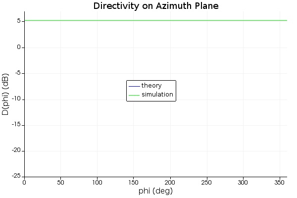
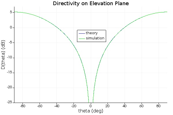
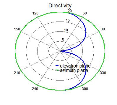
The script generates plots of the antenna’s directivity in the azimuth (X-Y) and elevation (Y-Z) planes and compare them to theory [1] ( Dϕ and the dominant Dθ polarization). The strong match between the FDTD and theory is evident, in which the directivity obtains a maximum value of 5.172 dB, which is very close (1%) to the theoretical directivity of 5.167 dB. The figure on right shows a polar representation of the monopole’s directivity pattern.
Radiation Performance
Simulation results generated in the script prompt using the script file quarter_wave_monopole.lsf are listed:
============Radiation Performance==============
Resonant Frequency: 2.13 GHz
Input Power: 6.53 nW
Accepted Power: 6.53 nW
Radiated Power: 6.49 nW
Radiation Efficiency from Input Power: 99.4 %
Radiation Efficiency from Accepted Power: 99.4 %
Maximum Directivity: 5.17 dB
Total Realized Gain: 5.15 dB
Please refer the script file for details for those quantities, which is at the end of the script. Definitions and explanations of those quantities can be found in the Methodology page.
Since the monopole antenna is lossless and of resonant size, its radiation efficiency with respect to accepted power is nearly 100%.
|
Note : Radiated Power The radiated power is calculated from the directivity analysis group but may need to be re-normalized to the input power. This is due to small normalization differences in the sourcepower script command and the amount of injected total power. In certain geometries where the port's fields can rapidly vary across the mesh grid, this is a necessary step to obtain accurate results. |
Related references
- C. A. Balanis, Antenna Theory and Design, 4th Edition. John Wiley & Sons (2016).