
Extracting the bandstructure for simulations with high loss may require some additional care in the setup and tuning of the simulation parameters because the field decay quickly which makes it challenging to locate the resonant modes of the system.
To demonstrate how to extract the bandstructure for simulations with high loss, here we show an example of a 1D-periodic chain of spheres made of a highly absorbing metal, with PML boundaries on four sides. bandstructure_1D.fsp contains the simulation set up according to the rectangular photonic crystal page and yet it does not yield a clear bandstructure diagram. bandstructure_1D_fixed.fsp has implemented some of the following solutions listed below, and results in a clear bandstructure plot. The bandstructure plots can be obtained by running the bandstructure_1D.lsf script file.
Problems associated with simulations with high loss
The fields decay more quickly when more loss is introduced, and the useful part of the time signal that is collected by the time monitors is shortened. The Fourier transform of the time signal becomes noisy, making it difficult to extract the resonance peaks.
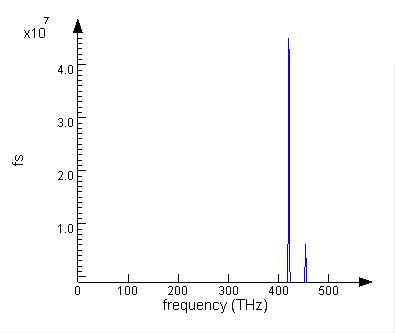
The following figures compare the sum of the Fourier transforms of the time monitor data, fs, at a particular k vector for the lossless square 2D simulation (left), and the lossy 1D-periodic chain example here (right). You can see that the signal from the simulation with low loss has sharper, narrower peaks and less noise than the signal from the simulation with high loss. This is why it is more difficult to obtain the correct resonance peaks for simulations with high loss.

Solutions
The following plots show the bandstructure diagram for the unmodified bandstructure_1D.fsp (left) and modified bandstructure_1D_fixed.fsp (right) simulation files based on the solutions listed below.


Source and monitor placement
If you are interested in looking at a particular mode or set of modes and you have an idea of what the field profiles of the modes should look like, you can choose to place the dipole sources in optimal positions and orientations for exciting those modes, while avoiding exciting modes that you are not interested in. In the example here, we are only interested in looking at the mode with strong fields between the spheres, so we place an x-oriented dipole source on the x-axis between the spheres.
Similarly, by choosing monitor placement one can also minimize the signal that is recorded from modes you are not interested in. In our example we have also placed the monitor on the x-axis.
Symmetry
You can use symmetry in the boundary conditions to isolate modes of interest. In our example, we are interested in a mode that is symmetric across the y and z axes. By setting the y and z boundary conditions to be symmetric, we eliminate any modes that do not satisfy this symmetry condition.
Apodization
The resonance that we are interested in may only occur for a short period of time and it may not occur at the center of the recorded time signal. To help determine which portion of the time signal to take the Fourier transform from, you can run a preliminary simulation and look at time monitor signal, or use a movie monitor to estimate the center time and duration of the resonance. You can then use this information to adjust the apodization window center and width settings in the analysis tab of bandstructure object.
Source spectrum
You can also adjust the source spectrum to ensure that more energy is coupled into the bands you are interested in. For example, if you are interested in the high frequency bands, you can adjust the source frequency center and bandwidth to the range that overlaps with the higher frequency bands. As a result, the strength of the resonance peaks in the Fourier transformed time signal from the higher frequency modes will increase relative to the lower frequency resonance peaks, allowing you to extract the higher frequency bands. In the example file that has been fixed, the minimum and maximum source frequencies have been set to match the apodization frequency range in the bandstructure object analysis tab variables.
Tolerance
It is also possible that you have a clean signal from which to extract the bandstructure but some of the points are being excluded from the bandstructure plot because the height of the resonance peak is below tolerance. If the bands can be seen clearly in a plot of fs vs k, then you will be able to extract more of the points in the bandstructure by lowering the tolerance setting in your analysis script.