This example shows how to add gain to the active region of a VCSEL laser.
Simulation setup
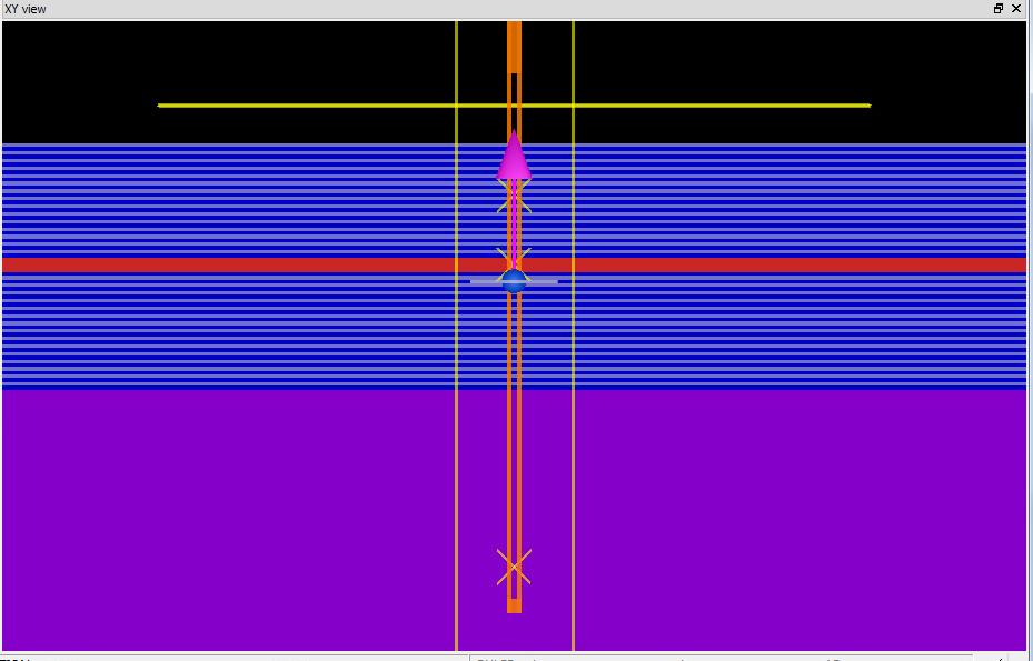
The above screenshot shows a 2D VCSEL laser simulation. We will add gain to the active layer (shown in red). The VCSEL layers of this example were designed to resonate at 850nm, or 353THz.
Results
First, we will study the system without gain. The active layer is defined as a simple dielectric with an index of 3.49. A plane wave source located near the active layer is used to excite the system.
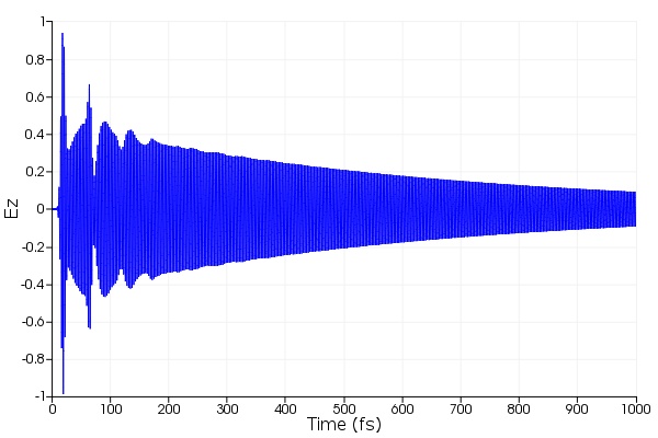

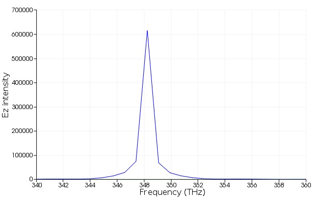
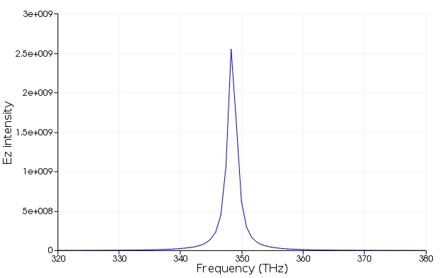
First, look at Ez vs time in the active layer from the time monitor "Monitor1". A slow decay is visible, due to light leaking out the top and bottom of the structure. We choose to terminate the simulation at 1000fs, for reasons that will become apparent when running the simulations with gain. An fft of the time signal shows that the structure does have a resonance at about 350THz, as expected.
We can also view the field profile with a 2D power monitor. When using profile or power monitors in simulations where the fields have not decayed to zero, it is important to use the apodization feature. More information regarding apodization can be found in the reference guide on the page describing the spectral averaging and apodization tab for frequency domain monitors.
Next, we can add some gain to the active layer material and rerun the simulation. We use the material "active_gain", which is a Lorentz type material with a negative Lorentz permittivity; this material is available in gain_VCSEL.fsp. The index of the active layer acquires a small negative imaginary component that will produce gain.
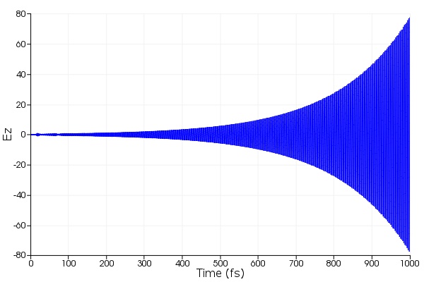
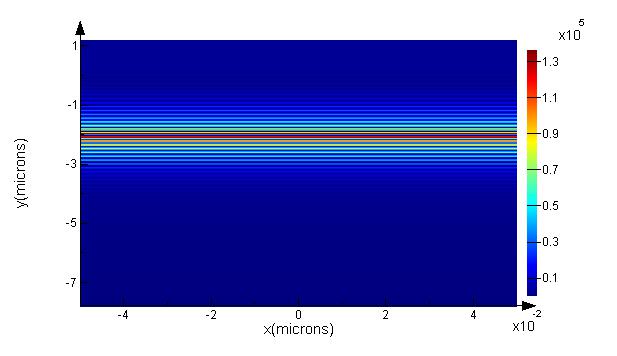
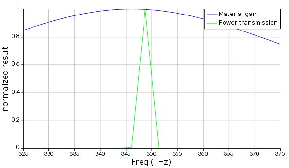
Once again, we look at the time signal. The behavior is very different now, with the fields growing exponentially in time. FDTD does not support a material saturation model, so the fields will continue to grow exponentially. The simulation must be terminated before the field values diverge. We choose to stop the simulation at 1000fs. Once again, the fft shows a strong resonance near 350THz. The field profile also looks quite similar, although much more intense. Finally, we can plot the power transmitted out of the top surface of the laser and the active region gain curve on the same figure using the script gain_VCSEL_trans.lsf. We can see that even though the material has broadband gain, we only see a strong amplification at the resonant frequency. An example that does include gain saturation is the 4 level 2 electron material model.