Simulating nonlinear effects in waveguides often requires long simulation times and propagation lengths. The 2.5D FDTD Propagator can simulate wave propagation over long distances efficiently, while still being able to accurately capture the interplay between the linear and nonlinear effects.
In this example, we will study four wave mixing (FWM) in a ring resonator based on a design in InP from reference [1], using the nonlinear Raman and Kerr Chi3 material model provided in the material database.
Linear Ring Resonator
We will start with the SOI ring resonator from MODE getting started example. First, a simulation without any nonlinear material is ran in order to find the location of the resonance peaks for this device. (If you are starting from ring_resonator_FWM.lms, simply disable the pump and signal sources, enable the broadband source and set the material of the ring resonator to "Si (Silicon) - Palik".) The script file ring_resonator_linear.lsf can be used to plot the transmission at the drop/through ports.

Fig.1 Results for the ring resonator without nonlinearity.
For the linear ring resonator, we find resonance peaks at ~1.506um, 1.533um and 1.560um as shown in Fig. 1
Nonlinear Ring Resonator
Now, instead of using "Si (Silicon) - Palik" as the material for the waveguide, we will switch to using the "Raman Kerr" material. Note that we have selected "Si (Silicon) - Palik" as the base material for the "Raman Kerr" model, with the "revert to base material for conformal mesh cells" option turned on (see Fig. 2b). This will allow us to incorporate the effect of linear material dispersion from Silicon on top of the nonlinear effects, as well as been able to benefit from conformal meshing even when using plugin materials.

(a)
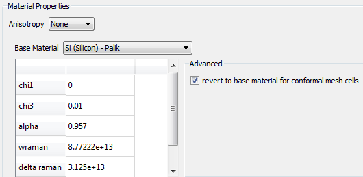
(b) Note that chi3 value shown here is more for demonstration purpose. Users are encouraged to use values and parameters suitable for their experimental setups.
Fig.2 Screenshots of the simulation setup: (a) layout editor and (b) properties of nonlinear material "Raman Kerr".
Next, we disable the "broadband" source and enable the "pump" and "signal" mode sources (at 1.534um and 1.561um respectively) positioned at the input port of the ring resonator. What we want to observe is the converted signal wave that results from the nonlinear interaction between the signal and pump waves. To do this, time monitors at the through and drop ports are set up to collect the time domain field data.
Note that under the Advanced options tab of the Propagator simulation region, we have chosen the "set simulation bandwidth" option and set the range to be from 1.45um to 1.6um. This will fix the simulation bandwidth for material fits, mesh generation, as well as time down sampling of monitors. This is especially important for nonlinear simulations because we are often interested in the response at wavelengths that are different from the source wavelength. We have also increased the simulation time to 50000fs. Typical nonlinear waveguide simulations will require longer simulation times and larger propagation lengths than simulations that only use linear materials.
The nonlinear simulation is also very sensitive to the shape of the injected mode and the fields in the gap regions between the waveguides and the ring. For these reasons we have included two mesh override regions ("mesh_top" and "mesh_bottom") that allow us to obtain appropriate field profiles for the pump and signal modes. Note that the E-field intensity profile for the pump source shown in Fig. 3a is slightly asymmetric without the mesh override region; when the mesh override is used, the mode becomes symmetric as expected (see Fig. 3b).

(a)

(b)
Fig.3 Comparison between E-field intensity of the mode injected by the pump source: (a) without mesh override and (b) with it.
With respect to the PML settings it is important to point out that we use the stabilized profile for the x direction. If the standard profile is used instead, the simulation diverges. For more details please visit the Diverging simulations page.
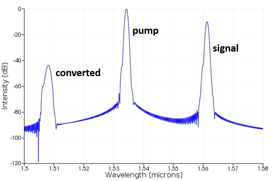
Once the simulation finishes running, we can use the ring_nonlinear_FWM.lsf script to plot the field intensity as a function of wavelength (see Fig. 4).
Fig.4 Spectrum of the field intensity for nonlinear simulation.
One can clearly see the pump and signal waves, as well as the converted wave at around 1.508um.
Related references
[1] C. Koos et al, FDTD-Modelling of Dispersive Nonlinear Ring Resonators: Accuracy Studies and Experiments, IEEE J. of Quantum Electronics, 42, 1215–1223, 2006
See also
Ring resonator (design and initial simulation)
Ring resonator (parameter extraction and yield analysis)
nonlinear Raman and Kerr Chi3 material model