In this example, we will consider how to use the Kerr nonlinear material model to simulate four-wave mixing.
Four-wave mixing
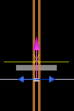
We will use a simulation setup that is very similar to the harmonic generation example, but for the material we use a third-order nonlinear medium (with Chi(3) set to 3e-18). Also, note that there are now three identical plane waves in the object tree, with the frequencies f1, f2, f3 = 100, 120, 140 THz respectively. You can enable or disable any of the sources by right-clicking on it in the object tree.
For this example, we will use a transmission monitor on top of the nonlinear medium to record the transmission. Note that instead of “use source limits”, we have to define a frequency/wavelength range large enough for us to see the harmonic generation. In addition, we cannot simply use the transmission script command since the normalization by the sourcepower will lead to additional noise. (The reason for this noise is that we are specifying a frequency range for the monitor that is much larger than the actual frequency range of the source; therefore, sourcepower will be close to 0 for the majority of the frequency range where the monitor is collecting data.) Instead, the script fourwave.lsf will calculate the transmission by integrating the Poynting vector over the monitor plane.
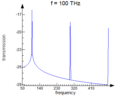
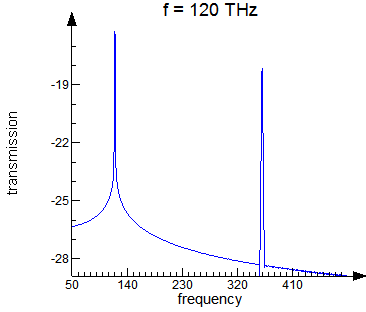
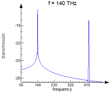
If you run the simulation with only one source enabled, you will see peaks at the 3rd harmonic frequency as shown in the figures below:
To determine the response of the medium due to a superposition of the three waves, enable all three sources in the Object Tree. Below is the transmission result with all sources enabled.
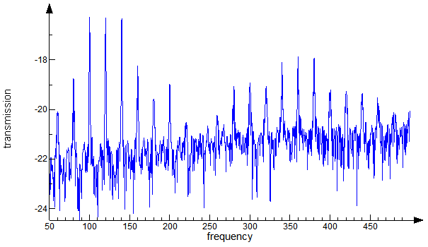
The additional peaks are formed by the interaction between the different wavelengths.
See also
Harmonic Generation, Kerr effect, Kerr nonlinear material model