
Numerical simulation results will never give exactly the correct answer; there is always some numerical error. It is important to understand some of the sources of numerical error and the steps that can be taken to reduce the error to an acceptable level. Reducing the error often involves increased simulation time and memory and so it is important to consider, for your application, what is an acceptable level of error so that you can run your simulations as quickly as possible. This page provides a thorough method for convergence testing of results from an EME simulation, so you can determine the possible sources of error in a simulation, and quantify the level of convergence.
Sources of error in an EME simulation
The following are some possible sources of error in an EME simulation. EME error diagnostics can be used to help quantify the error from these sources:
- The staircase effect in the longitudinal (propagation) direction. The longitudinal mesh is defined by the cells in the EME simulation region. If the cross-section of the structure or the material properties are continuously varying along the propagation direction, more cells will allow for a more accurate representation of the geometry in the longitudinal direction. Energy conservation can be applied and the CVCS subcell method can also be used in continuously varying regions to reduce the staircasing error.
- Number of eigenmodes used. The EME method relies on the modal decomposition of fields into a basis set of eigenmodes; we can specify the maximum number of these basis modes. In the limit where the number of eigenmodes is infinite, the amount of error associated with the EME calculation goes to zero. In reality, only a limited number of modes can be used in an EME calculation, since more modes mean longer simulation time and more memory. It is always a good idea to start with a small number of modes for the initial calculations and increase it as necessary until the result converges. With a large enough number of eigenmodes, even free space propagation can be simulated.
The following are some sources of error in an EME simulation that are also present in an FDTD simulation, and convergence testing for these properties is discussed in more detail in the FDTD convergence testing page:
- The staircase effect in the transverse direction. When dy and dz are finite, it is not possible to resolve geometric features to arbitrary resolution. Lumerical's conformal mesh can make convergence much faster for many geometries and materials, however, there will always be a geometric error for a finite-sized mesh. This error can be reduced by making the mesh size smaller, but eventually, other numerical considerations related to the finite precision of the numbers used will limit how small dy and dz can be.
If PML boundaries are used:
- The proximity of PML. If we are studying a mode that has evanescent fields, the PML will introduce errors if a non-negligible amount of the evanescent field comes in contact with the PML. For example, this will reduce the quality factor of a resonance or shift the frequency of a resonance.
- The reflection from the PML. The PML always has some reflection that can be theoretically calculated and changes with incident angle. Any reflection from the PML can re-interfere with the source, leading to incorrect power normalization, or simply re-interfere with the true scattered fields of the structure as they would exist in an ideal, unbounded space.
Convergence testing method
We can follow the steps described on the FDTD convergence testing page with additional tests for the number of modes used in each cell, and the number of cells used in a cell group region where the cross-section of the structure is continuously varying. We want to vary each parameter and quantify the level of convergence by measuring the difference with results from the previous step.
|
Note: that the convergence test for the number of eigenmodes can be done very efficiently with the mode convergence sweep tool. For this test, the modes have to be calculated only once for the desired maximum number of modes (see example in the next subsection). |
Example simulation
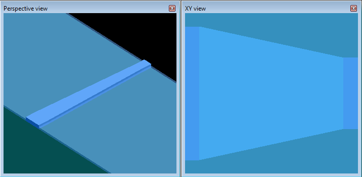
We will consider the [[pol_converter.lms]] simulation file, which simulates straight silicon ridge waveguides connected by a tapered region (see Polarization converter application example). The result we will consider is the conversion efficiency from the TE1 input mode to the TM0 output mode (ie. |S52|^2 of the user S-matrix result). Please see FDTD convergence testing for the types of metrics one can use to quantify the level of convergence.
The testing_convergence_EME.lsf script file performs convergence testing of the number of cells in the tapered region, the number of eigenmodes solved for in each cell, and the transverse mesh.
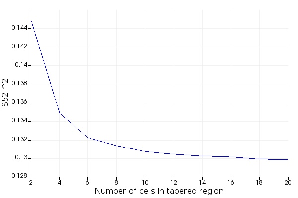
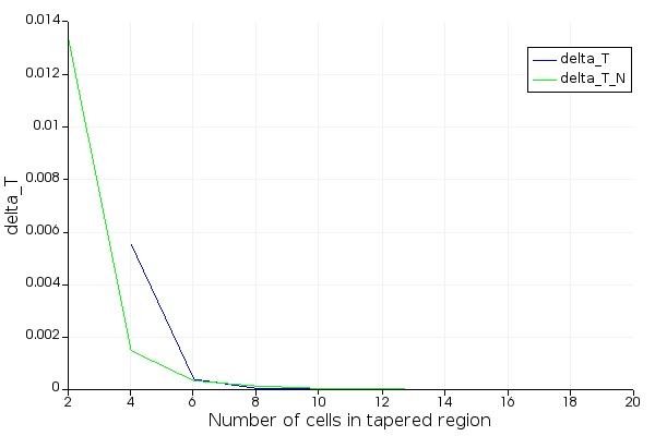
The number of cells to use in the tapered region is varied from 2 cells to 20 cells and the results are plotted below.
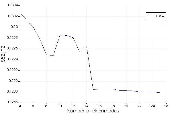
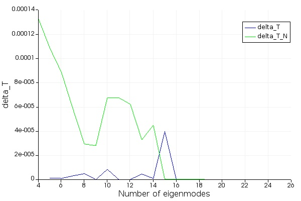
The number of modes solved for in each cell is varied from 4 to 25 and the results are plotted below. We use the mode convergence sweep tool.
The mesh step size of the transverse mesh set by the mesh override region was varied from 10 nm to 50 nm. Results are plotted below.
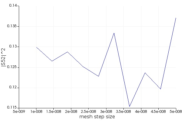

It turns out that for this particular example, the amount of error is relatively small even with the lowest settings for the number of cells and the number of modes in each cell (the number of cells in the tapered region contributing about 1% error and the number of modes contributing less than 0.015% error). For the transverse mesh, the amount of error goes up to about 2% for the coarser mesh step size, but the error goes down to less than 0.1% with a mesh step size of 10 nm.