Understanding EME error diagnostics

The EME solver can perform a number of error diagnostics making it possible to determine which cell interfaces are causing problems and may require a larger number of modes, better mesh resolution, or different energy conservation settings.

The error diagnostics are grouped into 2 categories: global and local. Global diagnostics measure the accuracy of all contributions to the S matrix as a whole, while local diagnostics measure the accuracy for the specific source that is selected in the EME analysis window. Some of the diagnostics are relatively fast to calculate while others take more time. You can choose to include fast or slow diagnostics when executing eme propragate.

When describing the examples below, we will refer to the taper example at Polarization converter.

Global diagnostics

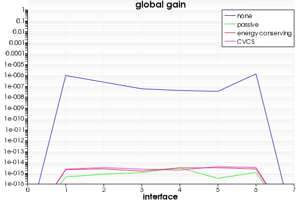
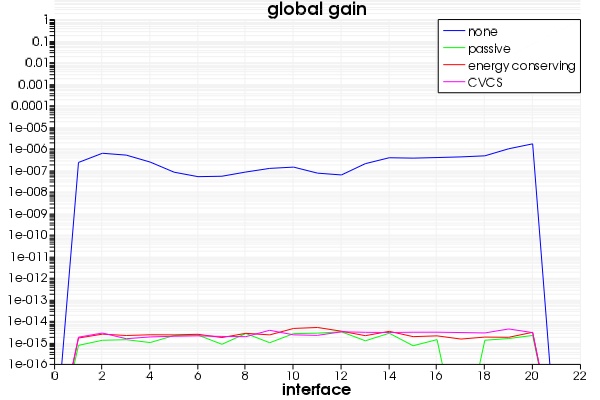
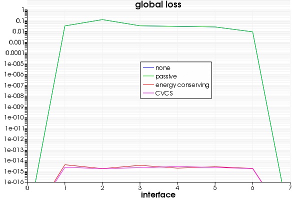
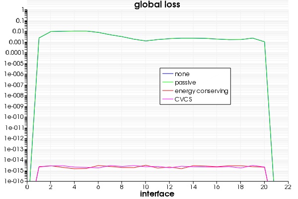
Loss and Gain. Here we calculate the maximum loss and gain violations that occur for each cell interface. In principle, the interface S matrix (the S matrix between the left and right hand modes of any given interface) should be energy conserving. This means that regardless of the incident field conditions, there should be no gain or loss of energy at the interface. In reality, because we have a finite number of modes calculated on a finite sized mesh, the interface S parameters will not necessarily conserve energy for all incident field conditions, and this diagnostic calculation gives the maximum possible violations that can occur. The data can be visualized as a function of interface number or as a function of x position (choose which in the Parameters section of the visualizer, under the tab 'Parameter'). When considering the interface positions, the first interface is 0 and the last interface is N where N is the number of cells. Therefore a violation at interface i-1 corresponds to the left interface of cell i, while a violation at interface i corresponds to the right interface of cell i. In general, we should see very small violations (particularly if we use the 'passive', 'conserve energy' or the CVCS method). However, if large violations are seen, it is worth also investigating the local errors because these global violations may result from excitation by very high order modes which would never be done in practice. The fast diagnostics option must be checked to update this result. These diagnostics are packaged in the result called 'global diagnostics'.

Expansion. The EME method is essentially an expansion of the modes on the left hand side of an interface onto the basis vectors formed by the modes on the right hand side, and vice versa. In principle, if we had an infinite number of modes, this expansion could be accomplished perfectly because each set of modes would be a complete representation of the entire vector space. In reality, we always have a finite number of modes and therefore we see the types of problems that are typical of, for example, expansion a function using a finite number of Fourier coefficients. This diagnostic simply expands each mode on the left hand side of the boundary using the basis vectors of all modes on the right hand side of the boundary (and vice versa), and measures the difference between the original mode and the expanded mode. If the modes on the left and right hand side are simply different representations of the same vector sub-space, this result will be 0. However, if the modes on either side represent different sub-spaces of the total space then this result will be potentially as large as 1. Typically the sub-spaces have some overlap and the result is between 0 and 1. If interfaces have a large expansion error, it may mean that you need to increase the number of modes on either side of the boundary. However, we should also consider some of the local error diagnostics because it is possible that only a small number of the modes are actually required for the desired source excitation. The fast diagnostics option must be checked to update this result. These diagnostics are packaged in the result called 'global diagnostics'.

Local diagnostics

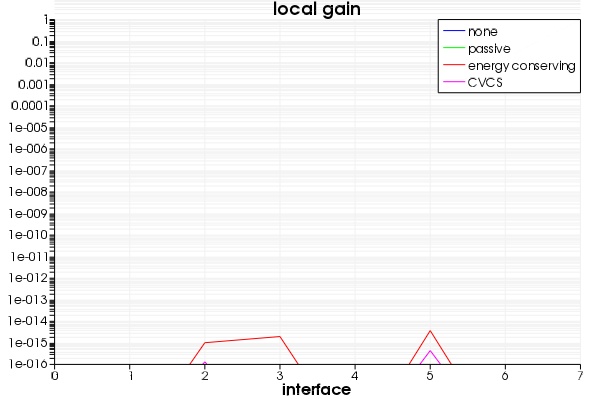
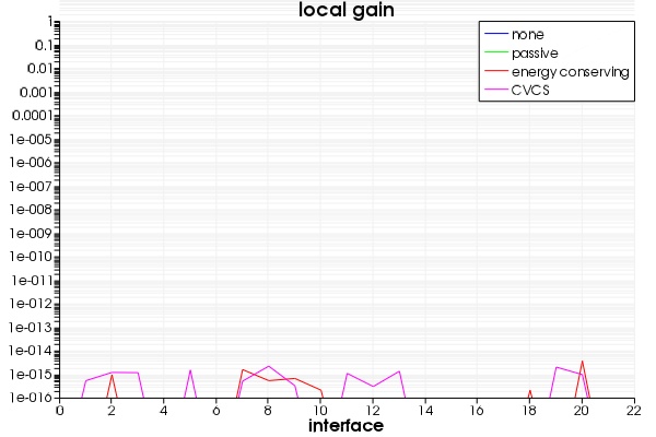
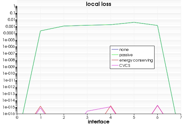
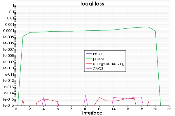
Loss and Gain. Here we calculate the actual loss and gain violations that occur at each interface for the given excitation source. These results may show much lower violations than the equivalent global results. These diagnostics are packaged in the result called 'local diagnostics'.

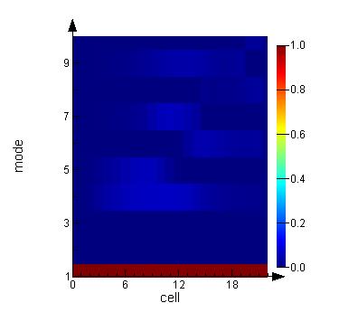
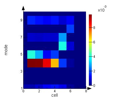
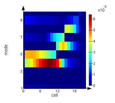
Coefficients. Here we show the forward and backward propagating coefficients for each mode in each cell, for the given source excitation. The coefficients are measured at the center of each cell. The port modes are included and are calculated at the port input and output positions. These coefficients are complex numbers in a matrix of size (N+2) X M where N is the number of cells and M is the maximum number of modes used in any cell (or port) of the EME region. If cells and ports use less than M modes, then the corresponding coefficients are simply set to 0. The data can be plotted vs cell number (with 0 corresponding to the left ports and N+1 corresponding to the right ports), or as a function of x position. These diagnostics are packaged in the result called 'coefficients'.

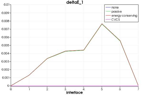
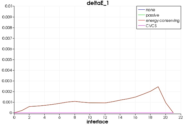
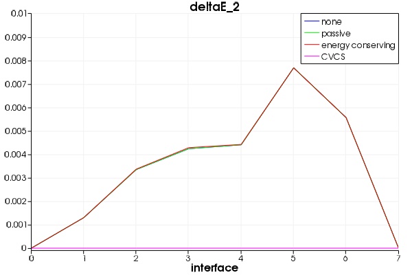
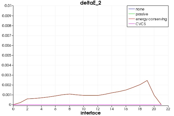
Field discontinuities. The EME method is fundamentally based on the continuity of the tangential E and H field components at each cell interface, which makes it possible to create a system of linear equations the solution of which gives the interface S matrix. Measuring the discontinuity of the tangential field components at the interfaces is a good way to see if enough modes are being used. These diagnostics are returned in the result called 'local diagnostics'. There are two results returned for the E field, which are

$$\Delta E_1=\frac{\int_{S}{\left|E_L^{||}-E_R^{||}\right|^2dS}}{\int_{S}{\left|E_S^{||}\right|^2dS}}$$

$$\Delta E_2=\frac{\int_{S}{\left|E_L^{||}-E_R^{||}\right|^2dS}}{0.5\int_{S}{\left|E_L^{||}\right|^2+\left|E_R^{||}\right|^2}dS}$$

where EL and ER refer to the left and right fields at each interface and ES is the E field of the excitation source at the port. There are two more equivalent results for the H field. These diagnostics are packaged in the result called 'local diagnostics' and are only calculated only when 'include slow diagnostics' is checked.

Directional Pmatrices

These EME error diagnostics are meant to provide a more intuitive quantification of how the forward and backward coefficients are contributing to the propagation by weighting them with the real power carried in these modes. This can be used to track mode scattering and identify problematic cells similar to global and local diagnostics.

forward_Pmatrix: For the diagonal of the matrix this is the forward power propagating in ith mode. The off-diagonal components provide the scattering between forward propagating modes resulting in a modification of total power.

Defined as a(i) * conj(a(j)) * P(i,j).

backward_Pmatrix: For the diagonal matrix this is backward power propagating in ith mode. For off-diagonal components it is the scattering between backward propagating modes resulting in modification of total power.

Defined asb(i) * conj(b(j)) * P(i,j).

cross_Pmatrix: The cross coupling indicates how forward modes scatter into backwards propagating modes. Unless strong reflections this will typically be quite small.

Defined as (-a(i) * conj(b(j)) + b(i) * conj(a(j))) * P(i,j).

combined_Pmatrix: Combining the three previously defined matrices into a single matrix, provides an overview of how the three mode scattering mechanisms effect the mode evolution. This is normalized, so summing over the real components should equal 1.

Defined as Cross Pmatrix (i,j) - Backward Pmatrix (i,j) + Forward Pmatrix (i,j).

Advanced settings and how to use them

There are three advanced settings in the EME solver that can have a significant impact on the results. These are:

• tolerance 1. This setting is used when solving for the S matrix at each interface. The interface S matrices are calculated from a linear system of equations that attempt to match the tangential E and H field components and the solution of these equations requires a matrix inversion. When there are modes on one side of the boundary that are not well matched by any modes on the other side of the boundary, the solution to the linear system of equations can result in S matrix coefficients that are much larger than 1 and do not conserve energy. This tolerance setting is used to eliminate coupling completely to modes that cannot be expanded on the other side of the boundary. Using values close to zero will result in smaller field discontinuties but can lead to large energy conservation violations that cannot be corrected without perturbing the entire S matrix. Using values close to 1 will make energy conservation work much better but can increase field discontinuities. For periodic structures where precise energy conservation is important, this value should typically be between 0.5 and 1. This setting affects the calculation of all interface S matrices, regardless of the choice of the "energy conservation" setting.
• tolerance 2. This settings is used to determine the maximum correction that will be made to a lossy interface S matrix to make it conserve energy. Ideally, all possible incident source conditions on an interface will result in perfect energy conservation. If the energy conservation setting is set to "conserve energy" then source conditions which result in loss are corrected to perfectly conserve energy. However, source conditions that result in a total transmitted and reflected power that is smaller than "tolerance 2" will be ignored which helps to avoid over correcting the original S matrix. For periodic structures where precise energy conservation is important, this setting should be quite small - typically 1e-5 or smaller - to ensure that no incorrect losses can occur.  This setting will only be used when the "energy conservation" setting is set to "conserve energy".
• tolerance 3. This setting is used for certain internal matrix calculations when trying to correct the interface S matrices to conserve energy or to be passive. It should be kept as small as possible, however, in some cases numerical errors can result if it is too small. In general, this setting should not have as much impact on the results as tolerance 1 and tolerance 2. This setting will only be used when the "energy conservation" setting is set to "conserve energy" or "make passive".

See EME - Advanced settings for more information.

Taper example

This example is based on the taper example at Polarization converter. We have run this example with only 5 cells in the middle cell group (the taper region) and 19 cells. The results for reach of the diagnostics, in four cases of energy conservation and CVCS settings (none, passive, energy conserving, CVCS) are shown in the table below. For ease of comparison, the line plots on the left and right side are shown on the same scale. The images are not shown with the same colorbar scale.

Diagnostic type	Result (5 cells in taper)	Result (19 cells in taper)
Global Gain
Global Loss
Local Gain
Local Loss
DE1
DE2
Forward coefficients (energy conservation=none)
Forward coefficients (CVCS)
Backward coefficients (energy conservation=none)
Backward coefficients (CVCS)
Expansion

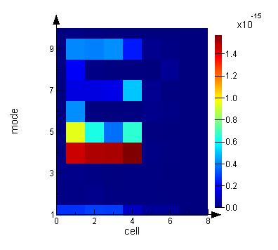
In the above results, since we have a taper region where the modes are not changing substantially from one cell to the next, we have no serious problems with local loss and gain or even with global loss and gain. However, setting the energy conservation to passive or energy conserving drives all global and local gains and losses to about 1e-15. The discontinuity in the electric fields is almost identical for both normalizations and shows that the largest discontinuity occurs near the end of the taper region. Note that the field discontinuities are exactly zero when CVCS is turned on. The forward coefficient magnitudes show that the light essentially propagates in the fundamental mode, but that some forward propagating higher order modes are important in the taper region. The backward propagating coefficients are extremely small for this device.

When the CVCS method is applied, we enforce field continuity and energy conservation - however the condition for applying the CVCS method is a continuously varying geometry where the modes do not change substantially from one cell to the next - therefore here we should be considering the expansion error and adding more cells if it is too large. We can see that the expansion error is substantially reduced when we go from 5 cells to 19 cells. In some cases, it may be useful to introduce more than one cell group over a taper to have a non-uniform distribution of cell sizes which ensures a uniform expansion error across the taper.

Unlike tapers, in structures with abrupt transitions, such as MMIs, there can be a trade off to be made between field discontinuity and energy conservations. Typically, to better conserve energy the field must become more discontinuous and vice versa.