This page provides a list of steps that one needs to pay attention to when working with lossy waveguides and fibers.
Check if the mode is bound
This is the first step that one should verify when a mode is suspected to be "leaky". In many cases, a bound mode can appear to be ill-confined, and one may want to use PML boundaries because of this. If we know that the mode we are looking for is bound, the standard procedure with metal boundaries should be use. In this case, using PML boundaries is unnecessary and may introduce other complications. (Please see Starting with metal boundary conditions for more information.)
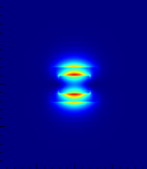
The best way to verify that a mode is bound is to use a 1D Eigenmode solver, and we will demonstrate this using the example file [[ridge.lms]]. When you first solve for the modes in this ridge waveguide, you will find the mode with neff ~ 3.475390. If you plot the "log" profile of the mode, it may seem that this mode is not bound at 1.55um.
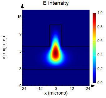
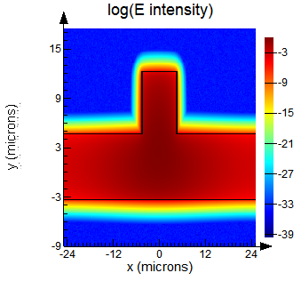
To verify wether this mode is bound or not, we can use a 1D mode solver to study the slab waveguide. Open the Edit window for the MODE simulation region, and change the solver type to "1D Y:Z prop", and change the "x" to -8. This will change the MODE region from a 2D solver to a 1D (linear y) solver. Here, we find the 2 modes with the highest neff to be a TE mode with neff = 3.475089 and a TM mode with neff = 3.475036. This means that any mode in the ridge waveguide that has an effective index greater than 3.475089 is bound (others will all leak away as slab modes).

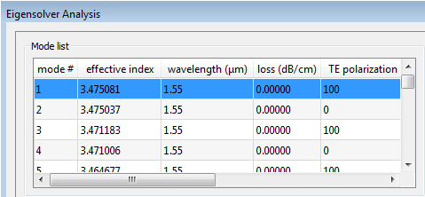
Because the mode at 3.475390 is bound, it is perfectly fine to use metal boundaries in this case. Note that we will still need to be careful and make sure that the metal boundaries are far enough away such that they are not influencing the modes. The best way to verify this is to increase the x-span and see if this changes the results significantly.
Use PML boundaries
If the waveguide/fiber does have radiative loss, then we will have to use PML boundaries. In this case, it is important to make sure that the PML boundaries are placed far enough away so that it does not interact with the evanescent tails of the mode. A distance of half a wavelength is a good start, but the best way to verify this is to increase the simulation region and see if this changes the result significantly.
Use a complex "n" value as an initial guess
The problem with leaky modes is that the imaginary part of the effective index can become quite large relative to the real part. In this case, if you use the search "near n" option with a real "n" value as the input, it will be difficult for the solver to locate the mode in the complex plane. The solution for this is to set a complex "n" value:
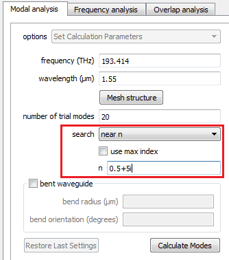
The closer you set this "guess" value to the real and imaginary part of the effective index of the desired mode, the easier it will be to find the mode. To do this, one can start with the last wavelength where a mode can still be found (ie. before the mode becomes too lossy), and then gradually move to the regime where the mode becomes lossy. The real and imaginary part of the effective index should change continuously, allowing us to guess what the next complex effective index should be.
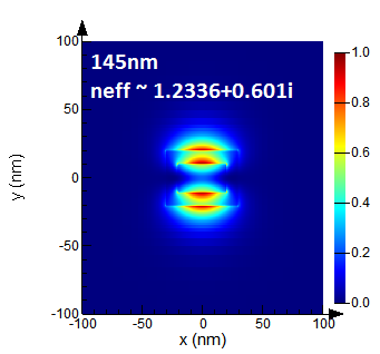
For example, in the file [[MIM.lms]], a mode with neff ~ 1.2336+0.601i can be found at 145 nm with the default "use max index" option.
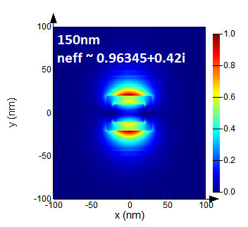
But if you use the same calculation parameters to look for the mode at 150nm, you will not be able to find the desired mode. In this case, it is much easier to find the desired mode by entering the neff found at 145nm (1.2336+0.601i) as the initial guess.
Loss conversion: dB/m (propagation loss) to \(\kappa\) (imaginary index)
An electric field propagating in the positive \(z\)-direction in a medium with a complex refractive index of \(n+i\kappa\) can be expressed as follows:
$$E(z) = e^{i2\pi(n+i\kappa)z/\lambda_0}$$
| [[NOTE:]] The \(\kappa\) in the above expression refers to the imaginary part of the complex refractive index, not the wavevector, \(k = 2\pi(n+i\kappa)/\lambda_0\). |
The propagation loss in dB/m for a mode propagating in the \(z\)-direction is defined as
$$loss = -10 \log_{10}(\frac{P(z)|_{z = \ 1\ m}}{P(z)|_{z = \ 0\ m}}) = -10 \log_{10}(\frac{|E(1)|^2}{|E(0)|^2})=-20 \log_{10}(\frac{|E(1)|}{|E(0)|})$$
Combining the formulas gives
$$loss = -20 \log_{10}(e^{-2\pi\kappa/\lambda_0})$$
Solving for \(\kappa\) gives
$$ \kappa = \frac{loss \cdot \lambda_0}{20 \cdot 2\pi \cdot \log_{10}(e)} $$