This page provides more information on the Modal Analysis part of the Eigensolver analysis window. Use the 'options' pull down to select the various types of analysis.
Set calculation parameters
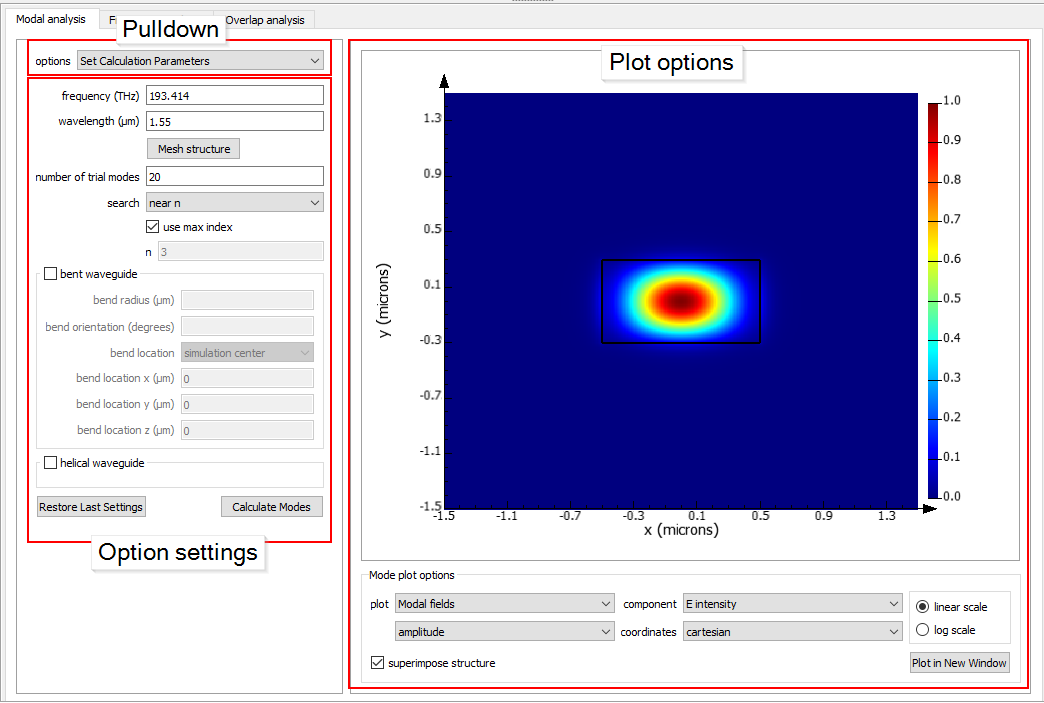
With the option pull-down box set to SET CALCULATION PARAMETERS, the modal analysis tab displays the calculation parameters. Some of the parameters can be set through the List of commands.
The parameters shown include:
- FREQUENCY: The frequency at which the modes are solved
- WAVELENGTH: The wavelength at which the modes are solved
- MESH STRUCTURE: Used to produce a mesh of the structure which can be examined in the visualization window
- NUMBER OF TRIAL MODES: This is the maximum number of modes returned in the Mode List. If there are less modes found, the number of modes in the Mode List will be smaller than this number.
- SEARCH: Define the target effective index value(s) for mode calculations
- USE MAX INDEX: Checked by default. If checked, search the modes that have the highest possible effective indices, the search results typically include the fundamental modes. Un-check this option to define N and find other modes.
- N: Search around a specific value of effective index. Users can type complex effective index values (ex. 0.5+5i), which is very useful for studying modes with high loss.
- NEAR N: Find all of the modes around a value of effective index
- IN RANGE: Find all of the modes within a range of effective index values defined by N1 and N2, with N1 > N2.
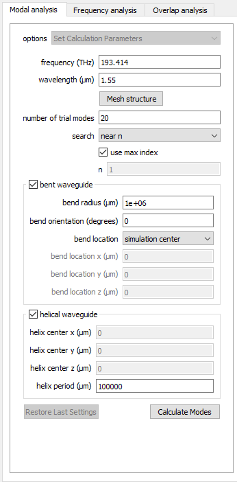
- BENT WAVEGUIDE: This checkbox is used to specify whether the waveguide is bent
- BEND RADIUS: The radius of curvature of the bend
- BEND ORIENTATION: The direction in which the waveguide is bent; refer to Bent waveguide calculation in User Guide for more details.
- BEND LOCATION: The location of the point used to define the bend radius. Often the center or outer edge of the waveguide. See Solving bent waveguides overview for more information. There are two options:
- SIMULATION CENTER: The center of the FDE simulation region, not including the boundary conditions.
- USER SPECIFIED: The user can select the bend location, using the coordinates BEND LOCATION X, BEND LOCATION Y, and BEND LOCATION Z. A bend location outside of the simulation region plane would be projected in the plane (e.g. a bend location with non-zero Z location would be projected to Z=0 if the simulation region is located on the X-Y plane)
- HELICAL WAVEGUIDE: This checkbox is used to specify whether the waveguide is helical.
- HELICAL CENTER X, Y, Z: This is the center position of the helix, ie, the coordinates of the point around which everything is twisted. This is not user editable at the current release.
- HELIX PERIOD: The pitch of the helix.
- CALCULATE MODES: Starts the calculation
- RESTORE LAST SETTINGS: Resets all the settings in this tab to those that were used to calculate the modes in the mode list.
Power and impedance integration
With the option pull-down box set to POWER INTEGRATION, the modal analysis tab displays the settings used to spatially integrate the power distribution of the calculated modes. It allows users to drag and draw a region for integration or define the region by the vertices using the GUI.
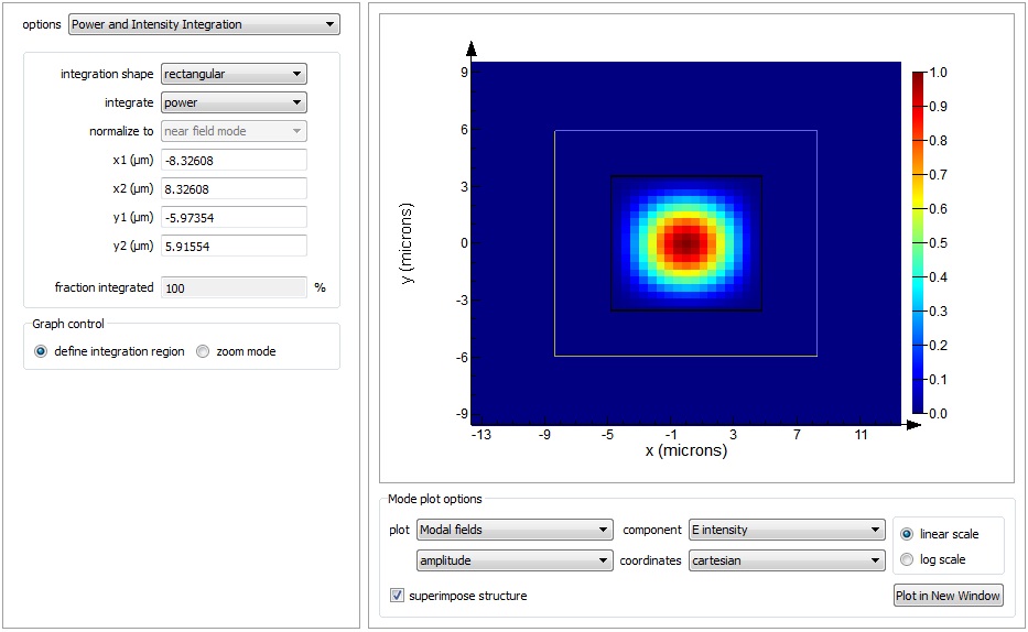
The power integration parameters are as follows:
- INTEGRATION SHAPE: Options include circular, rectangular and solid. The Solid option refers to any top-level geometry object (for example, a structure group, but not an object within a structure group) existing in the simulation. For overlapping geometries the mesh order is respected, otherwise they are resolved by tree order the same as in standard meshing.
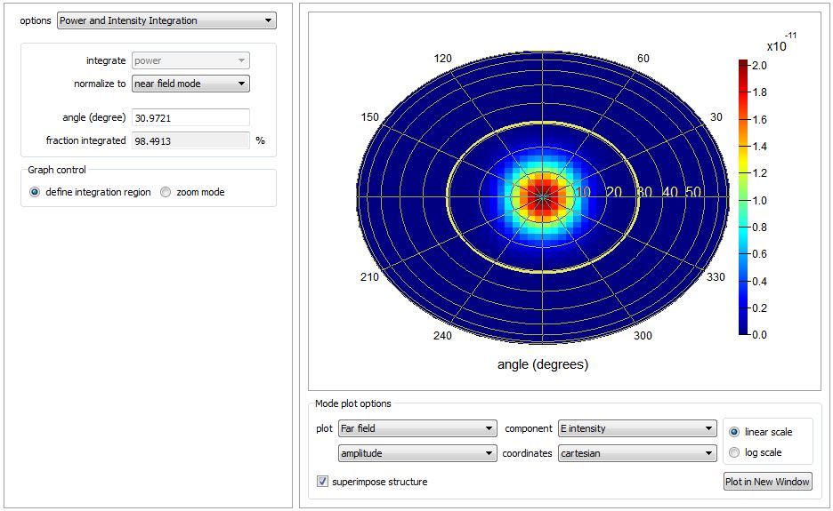
- INTEGRATE: Options include power, electric field intensity, or current (which returns the characteristic impedance). In the far field, only power integration is allowed so that the normalization to the near field mode is physically meaningful. Note that in the far field, the power is proportional the electric field intensity.
- X1, X2, Y1, Y2 (or Z1, Z2) (valid for rectangular integration): defines the vertices of a rectangle over which the quantity of interest is integrated
- CENTER X, CENTER Y (or CENTER Z), RADIUS (valid for circular integration): defines the center and radius of a circle over which the quantity of interest is integrated
- NORMALIZE TO (valid for far field only): Two options exist:
- NEAR FIELD MODE: Allows the user to normalize to the near field, or
- PROJECTION SURFACE: Allows the user to normalize to the total far-field quantity
- ANGLE (valid for far-field angular integration): defines angular cone over which the quantity of interest is integrated
- FRACTION INTEGRATED: The result of the integration procedure for power or electric field intensity integration options. This quantity updates itself as variations in the above parameters are made
- CHARACTERISTIC IMPEDANCE: The result of the integration procedure for the current integration option. This quantity updates itself as variations in the above parameters are made. The characteristic impedance is calculated using
$$ Z0 = \frac {P}{I^2} $$
Where P is the total power carried by the mode and I is the current calculated by integrating the H field around the outer edges of the integration region:
$$ I=\oint_{c} H \cdot d l $$
- GRAPH CONTROL:
- DEFINE INTEGRATION REGION: In this state, the mouse is used to graphically define the region over which the integration will be performed
- ZOOM: In this state, the mouse controls the zoom of the current figure in the visualization window
Far field settings
With the option pull-down box set to FAR FIELD SETTINGS, the Modal Analysis tab displays the settings used to project near field profiles into the far field.
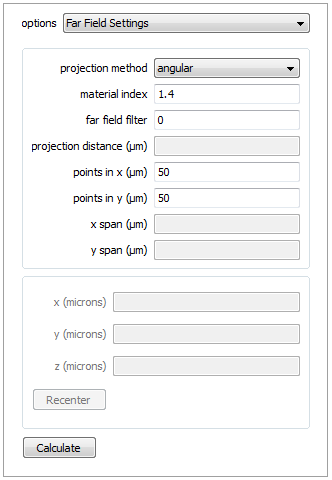
The following parameters are required:
- PROJECTION METHOD:
- ANGULAR: Projects the near-field into an angular coordinate system using a fully-vectorial, accurate algorithm. For slab waveguides, the far field information is plotted as a function of position. For waveguides with a two dimensional cross-section, it is plotted in polar coordinates.
- PLANAR: Projects the near-field into a Cartesian coordinate system using a fully-vectorial, accurate algorithm.
- MATERIAL INDEX: This field specifies the refractive index through which the far field projection is performed
- Z DISTANCE (only valid for planar projections): This field specifies the distance (in the units specified) to the projection plane
- POINTS IN X, Y (or Z): These fields allow the user to specify the number of points in the projection plane. The larger the number of points, the longer it will take to calculate the far field projection.
- WIDTH, HEIGHT (only valid for planar projections): the physical extent of the far-field plane, measured in the units specified
- X, Y, Z (only valid for planar projections): this specifies the center of the projection plane
- RECENTER: pressing this button will result in recalculation of the far-field projection, centered on the X, Y, Z values specified for the center location
- CALCULATE: this button will calculation of the far-field projection
Data export
The data export pull-down is where the user can save the calculated mode data to a file that can read in by another application for additional visualization or analysis.
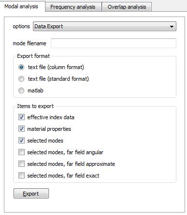
The data export options are as follows:
- MODE FILENAME: the filename to which the data will be saved. The file will appear in the same directory in which the simulation project appears.
- EXPORT FORMAT: these radio buttons are where the user specifies if they want the data saved to a text file, a Matlab-compatible file or a Lumerical .ldf file. The available options for the text file include column-formatted data, standard format data. For more information about the available options, consult the List of commands section.
- ITEMS TO EXPORT: these checkboxes allow the user to specify which part of the calculation data they wish to export. Options include:
- EFFECTIVE INDEX DATA: exports the real and imaginary effective index data.
- MATERIAL PROPERTIES: exports the vectors (1D) and matrices (2D) containing the permittivity (real and imaginary) and conductivity values for the x, y, and z directions.
- SELECTED MODES: exports the electric and magnetic field values in the x, y, z directions (i.e. Ex, Ey, Ez, Hx, Hy, and Hz) and vectors containing the x and y (or z) positions at which the values are calculated.
- SELECTED MODES, FAR FIELD ANGULAR: exports the far-field patterns of the electric field intensity in a polar coordinate system with x and y components of the unit vector defining the direction in which the values are calculated.
- SELECTED MODES, FAR FIELD APPROXIMATE: exports the far-field patterns of the electric and magnetic field values in the x, y, z directions (i.e. Ex, Ey, Ez, Hx, Hy, and Hz) and vectors containing the x and y (or z) positions at which the values are calculated.
- SELECTED MODES, FAR FIELD EXACT: exports the far-field patterns of the electric and magnetic field values in the x, y, z directions (i.e. Ex, Ey, Ez, Hx, Hy, and Hz) and vectors containing the x and y (or z) positions at which the values are calculated.
Mode plot options
The mode plot options allow changes in the plot shown above the options. In addition, you can use the PLOT IN NEW WINDOW button to create plots in a new figure window.
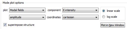
The plot options are:
- PLOT: There are two pull down menus which allow you to choose which data to plot
- COMPONENT: Choose the field component to plot. The options will change depending on whether the coordinates are Cartesian or spherical.
- COORDINATES: Specify whether the data is plotted on a CARTESIAN or a CYLINDRICAL coordinate system.
- LINEAR/LOG SCALE: determines whether the simulation data is plotted on a linear or a log plot
- SUPERIMPOSE STRUCTURE: toggles whether a black outline showing the physical structure is superimposed on the simulation data