This page discusses the physics of bent waveguides and provides details on the more complicated aspects of using the bent waveguide solver. With the exception of the Bend orientation setting section, which only applies to the FDE solver, the content on this page applies to both the FDE and FEEM solvers.
Bent waveguide physics
In a straight waveguide, the FDE/FEEM engine solves Maxwell's equations by looking for solutions in the form shown below:
$$E(x,y,z)=E_j(x,y)e^{i\beta_jz}$$
where \(\beta_j\) is the propagation constant of the \(j_{th}\) mode. It is a property of the mode and has units of inverse length. The effective index is generally used rather than propagation constant and it is defined by:
$$\beta_j=k_0n_{eff,j}$$
where \(k_0 = \omega / c\) is the wavevector in free space. Maxwell's equations are solved in a Cartesian coordinate system with the appropriate boundary conditions.
In a bent waveguide, the eigenmode solver will solve for modes of the form
$$E(\rho,\theta,y)=E_j(\rho,y)e^{i\widetilde{\beta_j}\theta}$$
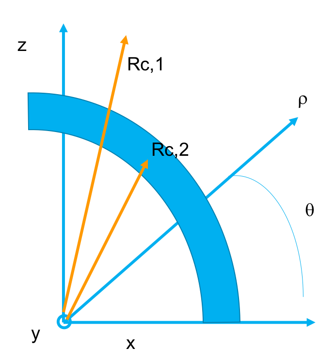
where \(\widetilde{\beta_j}\) depicts the angular propagation constant of the \(j_{th}\) mode and has units of inverse radian, and \((\rho,\theta,y)\) represents a cylindrical coordinate system as shown in the diagram below.

The effective index of the mode can be chosen as per relation below:
$$\widetilde{\beta}_j=k_0\widetilde{n}_{eff,j}R_c$$
where \(R_c\) is the bend radius. This definition provides a connection between the angular propagation constant (which describes the accumulated phase and loss per angle) and the regular propagation constant of a straight waveguide (which describes accumulated phase and loss per length). It is important to note that this definition of \( \widetilde{n}_{eff,j} \) depends on the choice of bend radius \(R_c\), as shown below. The angular propagation constant, on the other hand, is independent of \(R_c\), as long as the origin of the cylindrical coordinate system is the same. Therefore, we can relate the effective indices for two different choices of radius of curvature (with the same coordinate origin) according to:
$$\widetilde{\beta}_j=k_0\widetilde{n}_{eff,j,1}R_{c,1}=k_0\widetilde{n}_{eff,j,2}R_{c,2}$$
$$\widetilde{n}_{eff,j,1}R_{c,1}=\widetilde{n}_{eff,j,2}R_{c,2}$$
The bent waveguide solver reports \(\widetilde{n}_{eff,j}\) as the "effective index" (with its corresponding loss per length, "loss (dB/cm)") and \( \beta_j \) as the "angular propagation constant (1/rad)" (with its corresponding loss per angle, "angular loss (dB/rad)".
|
Note: Loss values The bend can lead to radiative losses, which can be measured by using Perfectly Matched Layer (PML) boundary conditions to absorb the radiation from the waveguide. The loss values reported by the solver are the net loss of the waveguide, not the loss due to waveguide bend only. |
Note that there is no unique definition for the bend radius of a waveguide. For example, the bend radius could be measured from the middle of the waveguide or the outside edge. This means that there is no unique definition for the linear effective index for a bent waveguide.
When using a MODE waveguide element in INTERCONNECT with imported bent waveguide mode data, the element uses the linear effective index and the waveguide length (which is the arc length for a bent waveguide). If you are consistent in your definition of the radius used to calculate the arc length (given by \(L = R_c\theta\), where \(L\) is the arc length and \(\theta\) is the angle subtended by the bend) this approach will work properly.
Bend radius setting
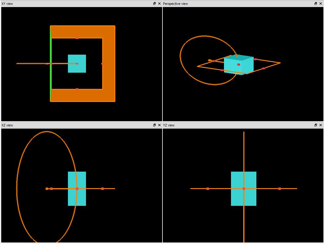
By default, the bend radius is measured from the center of the FDE/FEEM simulation region excluding the boundary condition regions as shown below:
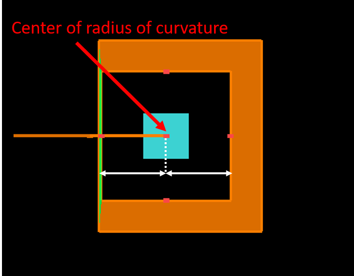
Users also have the option to select a user specified bend location anywhere within the simulation region. It should be noted however that a bend location outside of the simulation region plane would be projected in the plane (e.g. a bend location with non-zero Z location would be projected to Z=0 if the simulation region is located on XY plane).
|
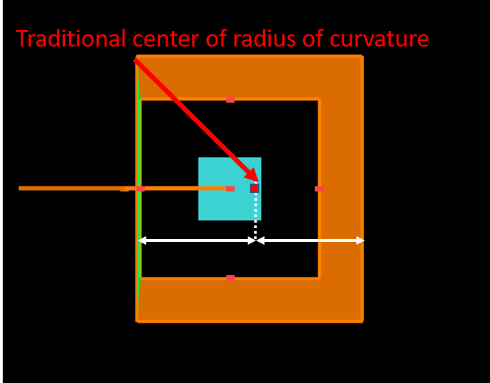
Note: Bent waveguide location before 2019A-R2 In versions of the software before 2019A-R2 (v7.13.1809) the bend location was fixed to be at the center of simulation region including the boundary conditions. This definition matches with the current one (for bend location at the "simulation center") as long as the width of the boundary condition regions is the same on both sides of the simulation. However, if the boundary conditions were to have different widths (e.g. metal on one side and PML on the other), then the center of the radius of curvature would be in a slightly different location, as shown here.
|
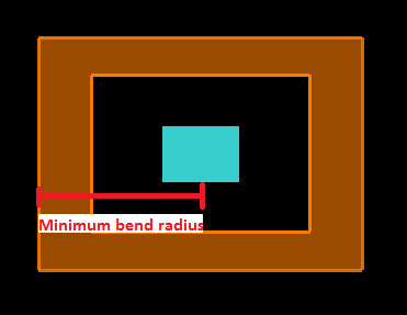
Minimum bend radius
The implied center of the radius of curvature must be outside the simulation region, plus the width of the boundary condition region. FDE/FEEM will automatically increase the bend radius if needed to meet this requirement. To maintain a smaller bend radius, the simulation region must be shifted or shrunk.
|
Note: Solver algorithm compatibility Bent waveguide solver is not available with "H transverse" solver algorithm. |
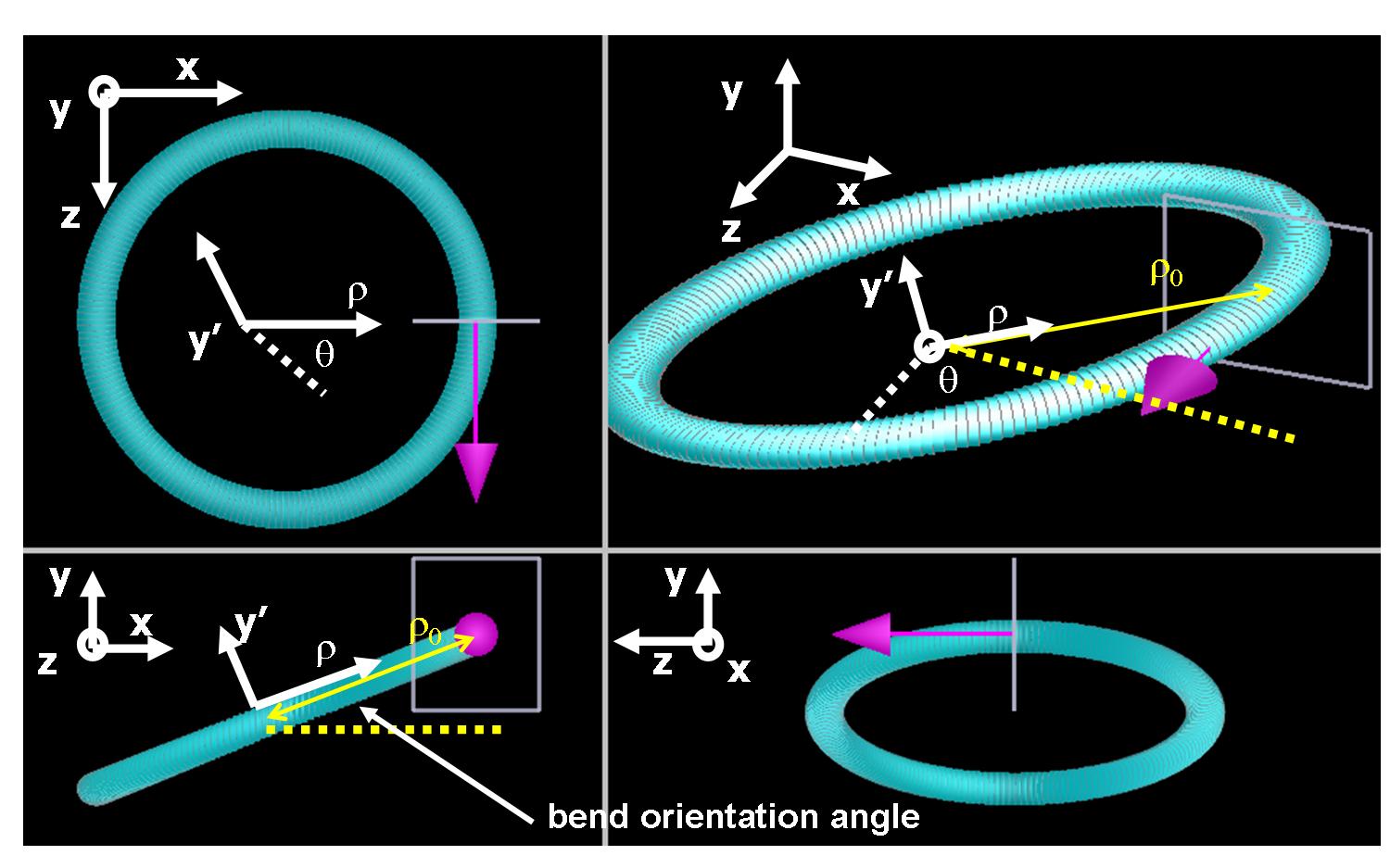
Bend orientation setting (FDE only)
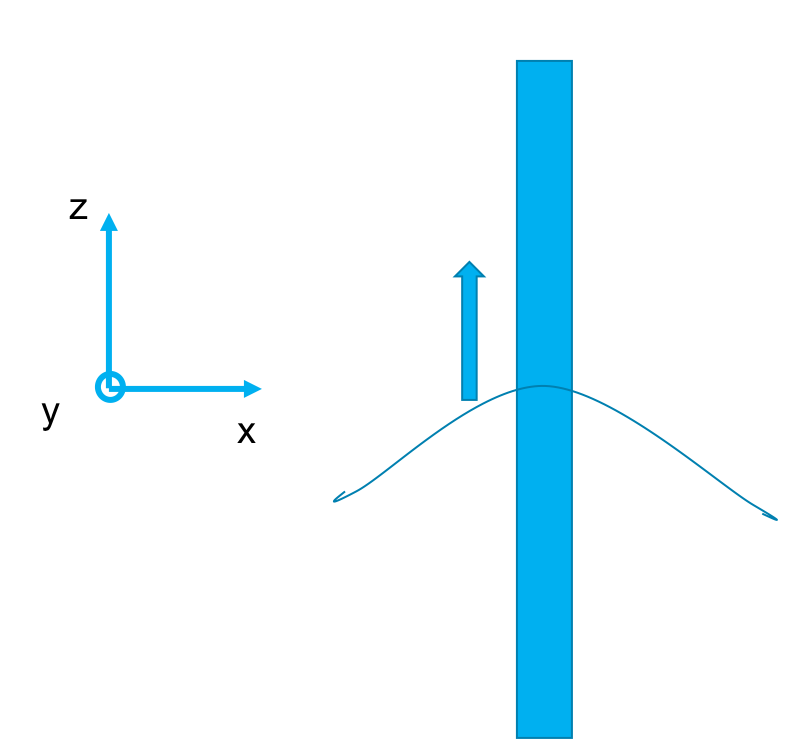
The (r,y',q) represent a cylindrical coordinate system shown in the figure below. The "bend orientation" angle, f, that can be set in the FDE analysis window is also shown in the following figure. The bend orientation angle determines the direction in which the waveguide bends. The cross section of the FDE simulation region is shown in white with a purple arrow indicating the direction of propagation of the mode. The FDE simulation region is the cross section of the waveguide when q = 0. The electromagnetic fields are returned in the Cartesian reference frame (x,y,z=0):
$$\vec{E}(\rho,y',\theta=0)=\vec{E}(x,y,z=0)=\left(\begin{array}{c}E_x(x,y)\\E_y(x,y)\\E_z(x,y)\end{array}\right)\\\rho-\rho_0=xcos(\phi)+ysin(\phi)\\y'=-xsin(\phi)+ycos(\phi)$$
Once the bent waveguide option is enabled, a glyph within the layout window would show how the bent waveguide curvature would look like with current bend settings. Users can take advantage of this to ensure correct bend settings before running the analysis.
To illustrate the effect of the bend orientation angle, the following images show the fundamental mode for a bent fiber with a circular cross-section in the XY plane.
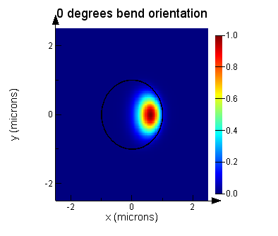
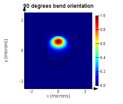
The left figure above clearly shows that the mode is distorted and shifted away from the center horizontally, since the bend is in XZ plane and the bend center is in the negative x side. Similarly, the right figure shows the mode center moves upwards when the bend orientation is set to be 90 degree.
FDE Solver in other orientations (XZ, YZ, or 1D solvers)
The above description assumes that you are using a 2D FDE solver oriented in the XY plane (meaning Z is the propagation direction). To understand the bend orientation for all eigenmode solver orientations:
- When the waveguide cross section is in the XY plane and Z is the propagation direction, if the bend is in the XZ plane around an axis parallel to Y, the bend orientation property is 0 when the bend center is in negative X, and the bend orientation property is 180 degrees when the bend center is in positive X; if the bend is in YZ plane around an axis parallel to X, the orientation is 90 degrees when the bend center is in the negative Y, and the orientation is 270 degrees when the bend center is in the positive Y; in the case that the bend is in between XZ and YZ planes, the orientation angle is in between;
- When the waveguide cross section is in the YZ plane and X is the propagation direction, if the bend is in XY plane, the orientation is 0 (negative Y) or 180 degrees (positive Y); in the XZ plane, the orientation is 90 (negative Z) or 270 (positive Z) degrees;
- When the waveguide cross section is in the XZ plane and Y is the propagation direction, if the bend is in YZ plane, the orientation is 0/180; in XY plane, the orientation is 90/270 degrees.
For the 1D Eigenmode solver, as long as the propagation direction is set, you can follow up the rules summarized above. For example, a 1D waveguide is in X axis and the propagation direction is Y, using the rule #3 we know that the bend orientation can only be in the XY plane, thus the bend orientation is 90 degrees. If the bend orientation is set to be 0 or 180 degrees, which means the bend is in YZ plane, because it is infinite in size (1D waveguide along X) , there is no effect to the mode.
To understand the bend orientation clearly, we suggest that you use the bent waveguide glyph to ensure the settings reflect the intended bend design.
See also
MODE - Finite Difference Eigenmode (FDE) solver introduction