This page describes three different methods for measuring reflectance from a structure. Using a monitor placed behind the source is the common and simplest method. Placing the monitor in front of the source can improve the accuracy in situations where there are source injection errors. We also discuss an alternative technique using a monitor placed along the source injection axis.
Monitor behind the source
The most straightforward setup technique used for measuring reflections from a structure is to place a frequency domain monitor behind the source injection plane. The incident and reflected fields exist in front of the source, but only the reflected fields will be measured if the monitor is placed behind the source.
|
Note: Direction of power flow If the net power flows in the negative direction, the transmission function will return a negative number. You may need to multiply by -1 if you want the these quantities to have positive values. |
Source injection errors
An ideal source would create a beam that moves in the propagation direction, without any scattering to other directions. Of course, FDTD is a numerical technique and some level of numerical error must be expected. In most simulations, these numerical source injection errors are negligible, meaning the method of placing a monitor behind the source to measure reflections generally works well. However, in some simulations, the source injection errors can be significant. These issues are more likely to occur when using a source that injects at an angle, a mode source, or a broadband source.
To understand the effect this back scatter can have on the accuracy of reflection measurements, imagine that 1% of the injected field is backscattered at the injection plane and 10% is actually reflected from the structure. In this case, the power measured by a monitor behind the source will be $$P=(0.01+0.1)^2=0.0121$$ for a source amplitude of 1. In other words, for this case, the error in the measured reflectivity is 2.1% even though the backscattered field is only 1%. Interference effects have been the two fields tends to amplify the effect of any source injection errors
Monitor in front of the source
If source injection errors are a problem in your simulation, you can measure reflected power using a monitor in front of the source.
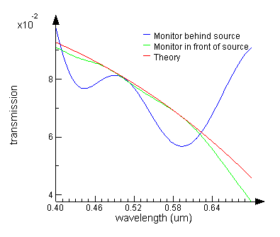
In the usr_relection_angled.fsp example file, a broadband plane wave source is injected with a center angle of 30 degrees. One power monitor is placed in front of the source and one is placed behind the source. By taking the reflection to be 1 minus the transmission from the monitor in front of the source, the reflection obtained from the monitor in front of the source is closer to the theoretical value than the reflection obtained using the transmission from the monitor behind the source. The usr_reflection_angled.lsf script plots the reflection using the two methods and the theoretical reflection.
|
Note: Monitor positions In a lossless simulation, the net power transmission through a monitor in front of the source is independent of its placement. The transmission will be the same whether it is placed between the source and the reflecting surface or past the reflecting surface. |
This technique for measuring reflection assumes that the injected power is normalized to 1. Source injection errors can also lead to errors in the power normalization. In such cases, it may be necessary to measure the actual power injected by running a reference simulation and then using this to re-normalize the results of your main simulation. To do this, use the monitor in front of the source to measure the forward propagating power in reference simulation that is setup exactly the same as the main simulation, but without the structure (which could lead to back reflections).
Line monitor interference technique
An alternative technique for measuring reflectivity is to use a line monitor placed along the source injection axis. This technique is not generally recommended because the analysis is more complex than the other methods, it will only work for cases where only a single mode exists, and the accuracy of the result is dependent on the spatial sampling rate.
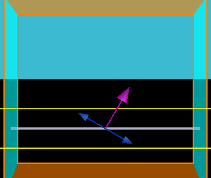
In reflection_interference.fsp, a plane wave in a vacuum is normally incident on a dielectric structure with index n=3. Between the source and the material interface, the amplitude of E^2 oscillates due to interference between the incident and reflected fields.
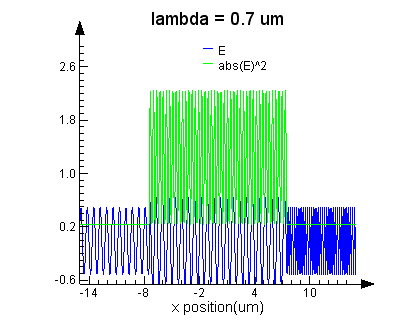
We can use the amplitude of E^2 in the region between the source and the interface to determine the power reflected:
$$ I(x) = I_1(x) + I_2(x) + 2 \sqrt{I_1(x)I_2(x)} \ cos(\varphi_1 (x) - \varphi_2(x) ) $$
I(x) will oscillate with amplitude:
$$ A(x) = 2 \sqrt{I_{1\ peak} I_{2\ peak}} = 2r$$
for incident intensity 1 and reflectivity \(R=r^2\)
Then,
$$ R = \left( \frac{A}{2} \right) ^2 $$
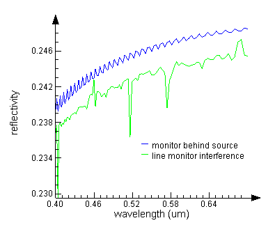
The following plots shows the calculated R using this technique from usr_reflection_interference.fsp and the measured transmission through a monitor behind the source. Low spatial sampling rate is a problem here because we cannot accurately measure the amplitude of the oscillation. Using a higher mesh accuracy setting, or adding a mesh override region would improve the accuracy of the result.