This page describes the apodization option of Frequency monitors. Apodization makes it possible to exclude effects that occur near the start and/or end of the simulation from the monitors fourier transform.
This feature can be useful for filtering away short lived transients that occur when a system is excited with a dipole source, and when studying high Q systems that decay very slowly. Apodization is considered to be an advanced feature and care must be taken when using it. Do some testing with a simple test simulation first, to make sure you understand how the monitor apodization affects your simulation results.
Monitor apodization applies a window function to the simulation fields E(t) before the monitor performs its Fourier transform of E(t) to obtain E(w). This makes it possible to calculate E(w) from a portion of the time signal. For example, start apodization can be used to ignore all transients which occur near the start of the simulation.
|
Note: Apodization will, in general, invalidate any source normalization performed and is therefore not suitable for accurate power or absolute field intensity measurement. For some resonant cavities, the absolute field intensities can be obtained with a bit of extra work. Details can be found in Correcting field amplitudes |
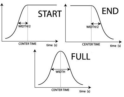
Full Apodization
This example shows how to use start apodization to get the correct mode profile for a photonic crystal cavity contained in usr_Tang_cavity.fsp. The simulation contains dipoles which are used to excite the modes of the cavity and a frequency monitor is set up to get the mode profile of the A11 mode.
Let's begin by looking at the electric field as a function of time. In particular, the blue line in the figure below shows |E|2 from the m2 time monitor. The transients at the beginning are due to all the energy injected by the dipoles which is not coupled into the A11 mode. For times greater than 600fs the time signal decays exponentially due to the fact that the majority of the energy left in the simulation is left in the cavity modes. The beating in the time signal is due to the fact that there are two cavity modes which are excited whose resonance frequencies do not lie far apart.
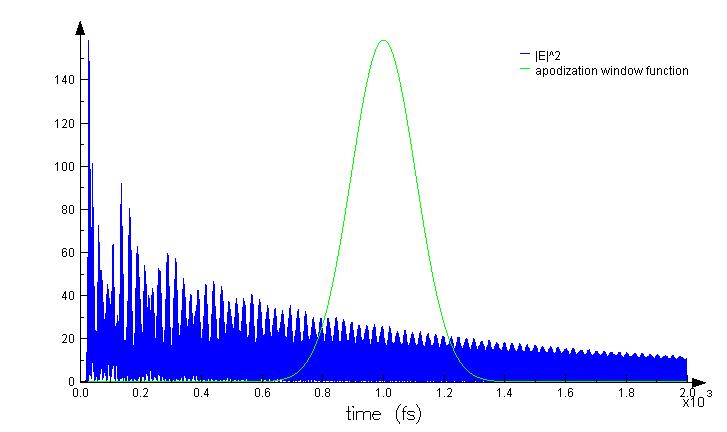
In order to plot mode profile for the A11 from a frequency monitor we need to use start apodization to get rid of the transients. The green line in the plots above shows the apodization window function used in the A11 monitor in the simulation. Note that the center time of the window function is set to 1000fs in order to ensure that most of the energy in the cavity is contained in the mode. The resulting mode profile is shown to the left below.
What happens if you do not use start apodization? The simulation contains a copy of the A11 monitor in which there is no apodization. This monitor is called A11_no_apodization. The magnitude of the electric fields are plotted in the image below to the right. In this image, you can see a superposition of the mode profile and the fields from the transients. The effect of the transients is most apparent at location of the sources.
Note that there are two sources in the simulation. They are placed at the origin of simulation and at x = 500nm, y = 400nm. However, since symmetry was used in the simulation the source at x = 500nm, y = 400nm is mirrored across the x and y axes. In the image below only three of the sources are pointed out (so that it is easier to see the mode profile).
|
Start Apodization 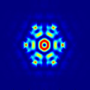 |
No Apodization 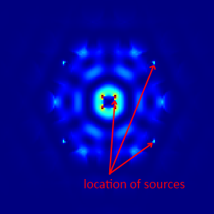 |
The end apodization does not have a visible affect in this simulation. To see that this claim is true, plot the electric field intensity from the A11_end_apodization monitor in the simulation. This monitor is the same as the A11 monitor except that it only uses end apodization, and the resultant |E|2 plot looks like the plot from the monitor without any apodization.