This page describes why it is best to start most Eigenmode Solver simulations with Metal boundary conditions (BC), even though PML boundaries may be the more obvious choice.
Description
In most simulations, the device substrate and other surrounding materials extend far beyond edge of the simulation. Therefore, the most obvious choice of BC's is PML, which will absorb fields at the simulation boundary. Metal BC's may seem like a poor choice because the real device is not surrounded by a metal box. In spite of this initial impression, we usually recommend starting with Metal BC's. Some simulations may eventually require PML, but a large fraction can be done entirely with Metal boundaries.
If the modal fields are very small at the edge of the simulation, then the choice of BC's is basically irrelevant (the BC doesn't matter when the field at the boundary is zero). In such cases, we can select the most numerically efficient BC, rather than the most physically correct BC. Metal boundaries have the following advantages over PML boundaries:
- Metal BC's make the simulation faster than PML.
- PML boundaries can introduce unphysical 'PML' modes.
- PML boundaries can introduce very small amounts of gain or loss in an otherwise lossless system.
As long as the modal fields are very small at the edge of the simulation region, Metal boundary conditions are usually the best choice. They will give the same result as PML, but the simulation will not suffer from the problems described above.
PML boundaries are required for modes that do extend to the edge of the simulation region. This is most likely to occur for modes that are not completely confined to the structure and have some radiative loss. For example, when studying bent waveguides, PML should be used because the bend can cause radiative loss.
Example
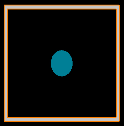
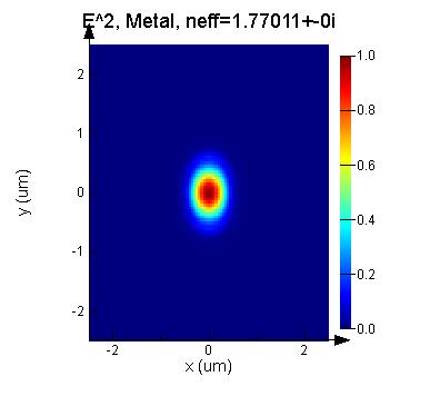
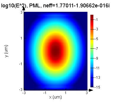
The associated file usr_start_metal_bc.lms has a very simple oval shaped waveguide. The script usr_start_metal_bc.lsf will calculate the effective index and mode profile of this structure using both Metal and PML BC's. As the following figures show, the mode profile and effective index from the two tests are very similar. However there are some interesting differences to notice:
- The Metal simulation runs much faster than the PML simulation.
- The mode profiles are slightly different, but these differences are only visible on a log scale. Some small differences are expected because the Metal BC's require that the fields go to zero at the edge of the simulation, while PML does not.
- The PML simulation shows that mode1 has a very small amount of loss (the imaginary part of the index). However, this value is numerically equivalent to zero.
|
Mode profile |E|^2 |
Mode profile log19(|E|^2) |
|
|
Metal BC |
 |
 |
|
PML BC |
 |
 |