This example demonstrates the feasibility of integrating Lumerical FDTD with Python using Application Programming Interface (API). In this example, we will set the geometry based on 2D Mie scattering example and then run the simulation using Python script. Once the simulation is finished, simulation results will be imported to Python, and plots comparing simulation and theoretical results as well as a plot of Ey intensity will be provided.
Requirements: Lumerical products 2018a R4 or newer
Note:
- Versions : The example files were created using Lumerical 2018a R4, Python 3.6 (and numpy), matplotlib 0.99.1.1, and Windows 7
-
Working directory : It should be possible to store the files in any locations as desired. However, it is recommended to put the Lumerical and Python files in the same folder in order for the above script files to work properly. It is also important to check the Lumerical working directory has the correct path, see here for instructions to change the Lumerical working directory.
- Linux: /opt/lumerical/interconnect/api/python/
- Windows: C:\Program Files\Lumerical\FDTD\api\python
During the Lumerical product installation process, a lumapi.py file should be automatically installed in this location.
This module is the key to enable Lumerical-Python API connection. Once the lumapi module is imported to Python, the integration should be ready. See this page for instructions for setting up Python API.
Note: Running Lumerical files from Python
If you already have the FDTD simulation or script files ready, you can run them from Python. For example, download the Lumerical script files ( nanowire_build_script.lsf and nanowire_plotcs.lsf ) and the nanowire_theory.csv text file and then run the script commands below in Python:
import lumapi
nw = lumapi.FDTD("nanowire_build_script.lsf")
nw.save("nanowire_test")
nw.run()
nw.feval("nanowire_plotcs.lsf")  # run the second script for plots
The commands above run the nanowire_build_script.lsf to set the geometry first, and then runs nanowire_plotcs.lsf to plot the simulation and theoretical results. These plots are created using Lumerical visualizer and will be identical to the plots in nanowire application example . In the rest of this page an explanation on how to build the geometry and analyze the results directly from Python will be provided.
Importing modules
The following script lines imports the modules ( importlib.util , numpy and matplotlib ) and the Lumerical Python API that will be used in the later script.
import importlib.util
#The default paths for windows
spec_win = importlib.util.spec_from_file_location('lumapi', 'C:\\Program Files\\Lumerical\\2020a\\api\\python\\lumapi.py')
#Functions that perform the actual loading
lumapi = importlib.util.module_from_spec(spec_win) #
spec.loader.exec_module(lumapi)
import numpy as np
import matplotlib.pyplot as plt
User can also use the method mentioned in the session management
Setting up the geometry from Python
The cross section results are wavelength dependent. To obtain the field profile for resonant mode we need to run two simulations: first simulation to calculate the resonance wavelength, and second simulation to adjust the wavelength of the profile monitor accordingly. Therefore, we define a function that sets the geometry and has profile monitor wavelength as an argument:
def runNanowireSimulation(profile_monitor_wavelength=1e-6):
    configuration = (
        ("source", (("polarization angle", 0.),
                    ("injection axis", "y"),
                    ("x", 0.),
                    ("y", 0.),
                    ("x span", 100.0e-9),
                    ("y span", 100.0e-9),
                    ("wavelength start", 300.0e-9),
                    ("wavelength stop", 400.0e-9))),
        #see attached file for complete configuration
   )
To set the geometry, we found that it is more efficient and cleaner to use nested tuple, however, advanced users may use any ordered collection. The order is important if a property depends on the value of another property.
    for obj, parameters in configuration:
       for k, v in parameters:
           fdtd.setnamed(obj, k, v)

    fdtd.setnamed("profile", "wavelength center", float(profile_monitor_wavelength))
    fdtd.setglobalmonitor("frequency points", 100.) # setting the global frequency resolution
    fdtd.save("nanowire_test")
    fdtd.run()
    return fdtd.getresult("scat", "sigma"), fdtd.getresult("total", "sigma"), fdtd.getresult("profile", "E")
Analyzing simulation and theoretical results
The script then calls the function to run the simulation, and then imports the simulation results into Python. Theoretical results are also imported from the nanowire_theory.csv file and interpolated over the simulation wavelengths:
nw = runNanowireSimulation() # recalls the function to run the simulation

## run the simulation once, to determine resonance wavelength
## and get cross-sections from analysis objects
sigmascat, sigmaabs, _ = runNanowireSimulation()
lam_sim = sigmascat['lambda'][:,0]
f_sim = sigmascat['f'][:,0]
sigmascat = sigmascat['sigma']
sigmaabs  = sigmaabs['sigma']
sigmaext = -sigmaabs + sigmascat

#load cross section theory from .csv file
nw_theory=np.genfromtxt("nanowire_theory.csv", delimiter=",")
nw_theory.shape
lam_theory = nw_theory[:,0]*1.e-9
r23 = nw_theory[:,1:4]*2*23*1e-9
r24 = nw_theory[:,4:7]*2*24*1e-9
r25 = nw_theory[:,7:10]*2*25*1e-9
r26 = nw_theory[:,10:13]*2*26*1e-9
r27 = nw_theory[:,13:16]*2*27*1e-9

for i in range(0,3):  # interpolate theoretical data
    r23[:,i] = np.interp(lam_sim,lam_theory,r23[:,i])
    r24[:,i] = np.interp(lam_sim,lam_theory,r24[:,i])
    r25[:,i] = np.interp(lam_sim,lam_theory,r25[:,i])
    r26[:,i] = np.interp(lam_sim,lam_theory,r26[:,i])
    r27[:,i] = np.interp(lam_sim,lam_theory,r27[:,i])
Plotting the results
One of the benefits of using the Lumerical Python API is that we can take advantage of the advanced Python modules. In this example, we use pyplot in the matplotlib module to plot the results.
The following commands plot the simulation and theoretical results for comparison.
plt.plot(lam_sim*1e9, sigmaext*1e9,label='sigmaext')
plt.plot(lam_sim*1e9, -sigmaabs*1e9)
plt.plot(lam_sim*1e9, sigmascat*1e9)
plt.plot(lam_sim*1e9, r25*1e9)
plt.xlabel('wavelength (nm)')
plt.ylabel('cross section (nm)')
plt.legend(['Extinction','Absorption', 'Scattering', 'r25 theory', 'r25 theory',
            'r25 theory'])
plt.show()

plt.plot(lam_sim*1e9, sigmaext*1e9,label='sigmaext')
plt.plot(lam_sim*1e9, -sigmaabs*1e9)
plt.plot(lam_sim*1e9, sigmascat*1e9)
plt.plot(lam_sim*1e9, r24*1e9)
plt.plot(lam_sim*1e9, r26*1e9)
plt.xlabel('wavelength (nm)')
plt.ylabel('cross section (nm)')
plt.legend(['Extinction','Absorption', 'Scattering', 'r24 theory', 'r24 theory',
            'r24 theory', 'r26 theory', 'r26 theory','r26 theory'])

plt.show()
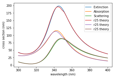
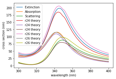
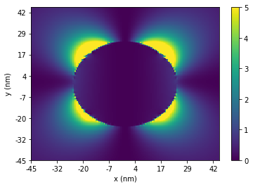
The above plots shows that the maximum extinction occurs near 348nm. This can be achieved by using numpy.argmax . To show the field profile at this wavelength, the wavelength of the profile monitor is adjusted and simulation is re-run for the second time using the commands below:
## run the simulation again using the resonance wavelength
_, _, E = runNanowireSimulation(profile_monitor_wavelength=lam_sim[np.argmax(sigmascat)])

## show the field intensity profile
Ey = E["E"][:,:,0,0,1]
Once the simulation is finished, we can extract the profile monitor results and plot |Ey|^2 at z=0:
  plt.pcolor(np.transpose(abs(Ey)**2), vmax=5, vmin=0)
  plt.xlabel("x (nm)")
  plt.ylabel("y (nm)")
  plt.xticks(range(Ey.shape[0])[::25], [int(v) for v in E["x"][:,0][::25]*1e9])
  plt.yticks(range(Ey.shape[1])[::25], [int(v) for v in E["y"][:,0][::25]*1e9])
  plt.colorbar()
  plt.show()