In some cases, it is interesting to understand if power is flowing forwards or backwards in a particular plane of a simulation. In this example, we show how this information can be obtained for a simulation with periodic or Bloch boundary conditions when there is a planar region of homogeneous, low-loss dielectric material.
This information cannot easily be determined from considering the Poynting vector alone. If we consider a simple example of a plane wave incident upon a perfectly reflecting boundary, the Poynting vector and the total transmitted power through a plane will be zero because the total normalized transmitted power is 1 (incident wave) - 1 (reflected wave) = 0. This is not easy to distinguish this from the case of zero fields everywhere, which also gives a total normalized transmitted power of 0.
In this example, we use the power direction analysis object which uses farfield and grating projections to decompose the measured E and H fields onto a basis state of forward and backward propagating plane waves. The forward power is then calculated by summing the power in all the forward propagating plane waves, and similarly for the backward propagating power. This method has some numerical errors that are largest when we have plane waves propagating at very steep angles to the measurement plane. For this reason, the forward transmission minus the backwards transmission may be different from the net transmission, measured simply by integrating the Poynting vector, by a few percent. The power direction object can be inserted from the object library in the optical power section.
Example
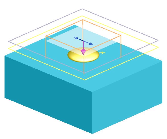
In this example, we consider light incident in a medium of dielectric index 1.4. The light propagates towards a gold ellipsoid on a substrate of index 2. Periodic boundary conditions are used, meaning that we are considering the light incident on a periodic array of these gold nanoparticles. The period is 1 micron in both x and y. We place a special analysis group for this calculation between the source and the particle so that it measures both the incident and reflected field. For the purpose of testing, we also place a reflection monitor behind the source. The analysis group contains a planar power monitor and also a small index monitor because it is necessary to know the refractive index where the fields were measured. It is important to note that this calculation is only valid if:
- The imaginary part of the refractive index is very small or zero. We ignore the imaginary part in this calculation.
- The material is completely uniform over the plane where the monitor is recording the field.
- Periodic or Bloch boundary conditions are used. This method could be extended to cases where PML is used as long as the fields go to zero near the edges of the simulation. Please contact Lumerical support if you would like to explore this case.
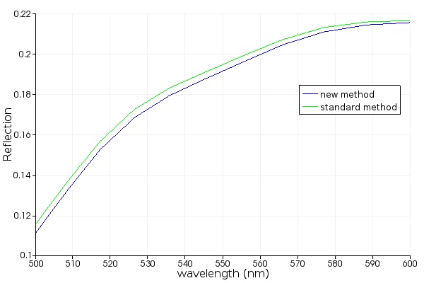
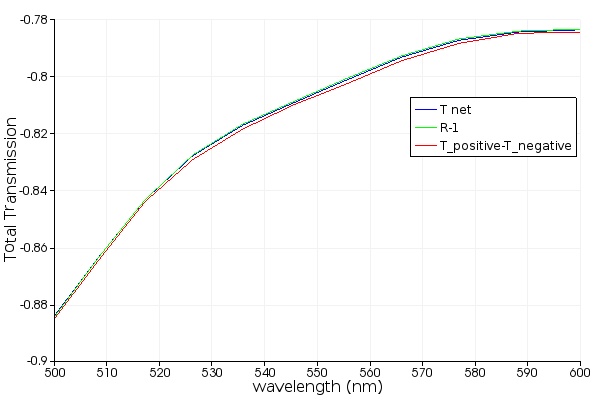
After running the simulation usr_power_direction.fsp , please run the script usr_power_direction_test.lsf . This analysis can take about a minute because there are a large number of far field projections involved and we record data at several different wavelengths - a new farfield projection is required for each wavelength. The script will create two figures. The first figure shows the reflected power measured using the power direction group, which is placed between the source and the nanoparticle. We see that we have successfully calculated the amount of backward propagating power ("new method"), which is close the reflected power measured in the usual way ("standard method"), although there is a small numerical error. The second figure compares the total transmission through the monitor measured in 3 ways:
- by using T_total, calculated from the transmission function
- by calculating R-1 where R is the reflection calculated in the usual way
- by taking the difference of T_positive and T_negative
We see that all methods agree reasonably well, but there is the largest error in T_positive-T_negative because this method involves the plane wave decomposition that introduces some more numerical error.