The near to far Grating Projections (GP) calculate the far-field profile from a periodic grating structure. The near field data is typically obtained from Lumerical's FDTD. The far-field is then calculated as a post-processing step.
A simple way to understand grating projections is to view them as a decomposition of the near field data using a set of plane waves propagating at different angles as the basis for the decomposition. The end result is that the far-field projection functions provide a straightforward and numerically efficient method for calculating the EM fields in the far-field region.
If your structure is not periodic, see the far-field projections page. If you're using DGTD or FEEM, see grating projections in DGTD.
Grating physics
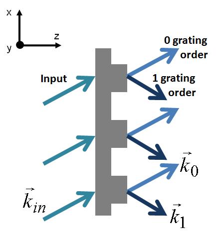
The grating functions are used to calculate the direction and intensity of light reflected or transmitted through a periodic structure. For example, the grating order directions of a 2D grating can be calculated from the well known grating equation
$$m\lambda=a_x(sin\theta_m+sin\theta_i)$$
where \(m\) is an integer, \(a_x\) is the periodicity of the grating in the \(x\) direction, \(\theta_m\) is the angle of propagation for the grating order, and \(\theta_i\) is the angle of propagation of the incident light.
For our purposes, it's more convenient to re-write this equation in terms of the wave vector k:
$$(\overrightarrow{k}_m)_x=(\overrightarrow{k}_{in})_x+m\frac{2\pi}{a_x}$$
where \(\overrightarrow{k}_m\) is the wavevector of the \(m\)th grating order and \(\overrightarrow{k}_{in}\) is the wavevector of the incident light, and the \(x\) subscript denotes the component of the wavevector.
In 3D, these equations become:
$$(\overrightarrow{k}_{n,m})_x=(\overrightarrow{k}_{in})_x+n\frac{2\pi}{a_x}\\(\overrightarrow{k}_{n,m})_y=(\overrightarrow{k}_{in})_y+m\frac{2\pi}{a_y}$$
where \(k_{n,m}\) is the wavevector of the \((n,m)\) grating order, \(a_y\) is the grating period in the \(y\) direction and (\(n\),\(m\)) are any integers that satisfy the condition
$$\mid\overrightarrow{k}_{n,m}\mid\leq k=2\pi\cdot index/\lambda_0$$
where \(index\) is the refractive index of the medium in which the grating order is propagating and \(\lambda_0\) is the vacuum wavelength.
It's important to remember that the grating order directions are defined entirely by the device period, the source wavelength and angle of incidence, and the background refractive index. In principle, the grating order directions can be calculated without running a simulation. However, in practice, the simulation must first be meshed in order for these functions to obtain necessary information such as the dimensions and period of the structure. The functions gratingn , gratingm , gratingu1 , gratingu2 , gratingangle can be used to calculate the direction of each order.
After running a simulation, the grating commands can be used to calculate the fraction of power that is scattered in each direction. The grating function uses a technique similar to a far-field projection to calculate what fraction of near field power propagates in each grating order direction. To get polarization and phase information, use gratingpolar and gratingvector.
Related publications
- Allen Taflove, Computational Electromagnetics: The Finite-Difference Time-Domain Method. Boston: Artech House, (2005).
- John B. Schneider, Understanding the Finite-Difference Time-Domain Method, Chapter 14: Near-to-Far-Field Transformation, (2010).
See also
- Far-field projection in FDTD
- Grating projection script commands
- Grating order transmission analysis object
- Understanding direction unit vector coordinates
- Understanding field polarization in the far-field
- Using grating projections to calculate fields at an arbitrary location
- Calculating magnetic fields in the far-field
- Projection distance scaling