 This page goes over the problems associated with direct simulation of temporal incoherence, the recommended simulation method, and provides an example simulation.
Problems with direct simulation
The phase, φ, of the light shifts randomly over time, on a time scale τc. For light near visible wavelengths, we have
$$ \vec{E}(t)=\vec{E}_{0} \cos (\omega t+\varphi(t)) $$
$$ T=\frac{2 \pi}{\omega} \approx 10^{-15} S $$
$$ \tau_{c} \approx 10^{-11} s $$
Even without random phase shifts, if the light is not monochromatic, it is incoherent.
In either case, the coherence length of the system is often much longer than any standard simulation time (τc>>T), so it is not efficient in general to directly model temporal incoherence. It is not possible to perform near to far field projections of incoherent results in the near field.
Recommended simulation method
By default, the frequency domain (DFT) monitors of FDTD return the monochromatic response of the system.
There are some advanced features to directly extract incoherent results (ie. where the value of Δf ~ 1/τc can be specified) - see Spectral averaging for more detail.
In general, the best approach is to calculate the monochromatic (or CW) response first, then calculate the incoherent result with
$$\left\langle\left|\vec{E}\left(\omega_{0}\right)\right|^{2}\right\rangle=\int W(\omega)|\vec{E}(\omega)|^{2} d \omega$$
where \( W(w)\) is the spectrum of the physical source used.
Temporal Incoherence Example
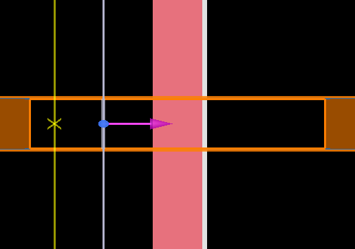
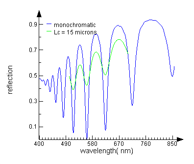
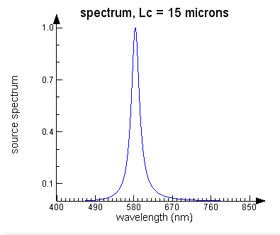
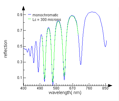
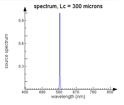
In usr_temporal_incoherence.fsp, we simulate the reflection from a 50 nm film of silver on a 500 nm slab of silicon. The associated script file, usr_temporal_incoherence.lsf uses the monochromatic results from the simulation to calculate the incoherent results (between 500 and 700 nm) for coherence lengths of 15 um and 300 um for a physical source with a Lorentz function spectrum. The resulting plots are shown below.
 |
 |
 |
 |