Plane wave and beam source - Simulation object – Ansys Optics

FDTD MODE

Plane wave sources are used to inject laterally-uniform electromagnetic energy from one side of the source region. In two-dimensional simulations, the plane wave source injects along a line, while in three-dimensional simulations the plane wave source injects along a plane. It is also possible to inject a plane wave at an angle. The plane wave source is actually the same object as the Gaussian source, with the only difference being the SOURCE SHAPE setting. Periodic or Bloch boundary conditions should be used with Bloch/periodic type plane wave source. Diffracting plane wave source can be used with PML in all directions. When a broadband result at angled plane wave incidence is pursued with one simulation without using Bloch BCs, the BFAST source technique should be used, please read more on BFAST plane wave.

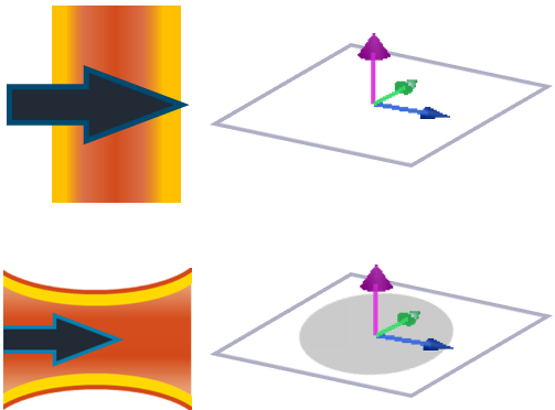
A Gaussian source defines a beam of electromagnetic radiation propagating in a specific direction, with the amplitude defined by a Gaussian cross-section of a given width. By default, the Gaussian sources use a scalar beam approximation for the electric field which is valid as long as the waist beam diameter is much larger than the diffraction limit. The scalar approximation assumes that the fields in the direction of propagation are zero. For a highly focused beam, there is also a thin lens source that will inject a fully vectorial beam. The cross-section of this beam will be a Gaussian if the lens is not filled, and will be a since function if the lens is filled. In each case, the beams are injected along a line perpendicular to the propagation direction and are clipped at the edges of the source.

NOTE: The following changes have been made to the polarization arrows in 2020 R.1.4 to avoid ambiguity with the polarization orientation.

Use a single-headed arrow corresponding to the initial polarization of the electric field
Add a green arrow for the polarization of the magnetic field

These changes affect only the way the source objects look in the GUI. The simulation results won't be affected in any way.

General tab

SOURCE SHAPE: The shape of the beam. It can be changed to a Gaussian, plane wave or Cauchy/Lorentzian.
AMPLITUDE: The amplitude of the source as explained on the Units and normalization page.
PHASE: The phase of the point source, measured in units of degrees. Only useful for setting relative phase delays between multiple radiation sources.
PLANE WAVE TYPE: Sets the type of the plane wave source. More information about each source type is available in dedicated topic available from "See also" section above. This menu is available for plane wave source only.
INJECTION AXIS: Sets the axis along which the radiation propagates.
DIRECTION: This field specifies the direction in which the radiation propagates. FORWARD corresponds to propagation in the positive direction, while BACKWARD corresponds to propagation in the negative direction.
ANGLE THETA: In 3D simulations, this is the angle of propagation, in degrees, with respect to the injection axis of the source. In 2D simulations, it is the angle of propagation, in degrees, rotated about the global Z-axis in a right-hand context, i.e. the angle of propagation in the XY plane.
ANGLE PHI: In 3D simulations, this is the angle of propagation, in degrees, rotated about the injection axis of the source in a right-hand context. In 2D simulations, this value is not used.
POLARIZATION ANGLE: The polarization angle defines the orientation of the injected electric field, and is measured with respect to the plane formed by the direction of propagation and the normal to the injection plane. A polarization angle of zero degrees defines P-polarized radiation, regardless of the direction of propagation while a polarization angle of 90 degrees defines S-polarized radiation.

Geometry tab

The geometry tab contains options to change the size and location of the sources.

Frequency/Wavelength tab

The Frequency/Wavelength tab is shown below. This tab can be accessed through the individual source properties or the global source properties. Note that the plots on the right-hand side of the window update as the parameters are updated, so that you can easily observe the wavelength (top figure), frequency (middle figure), and temporal (bottom figure) content of the source settings.

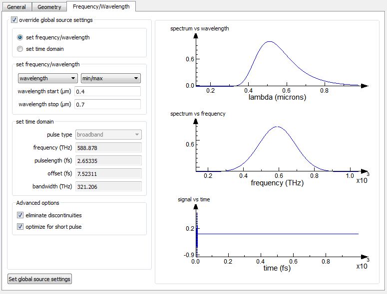
At the top-left of the tab, it is possible to chose to either SET FREQUENCY / WAVELENGTH or SET TIME-DOMAIN. In most simulations, the 'SET FREQUENCY / WAVELENGTH ' option is recommended.

If you choose to directly modify the time domain settings, please keep the following points in mind:

PULSE DURATIONS: Choose a pulse duration that can accurately span your frequency or wavelength range of interest. However, very short pulses contain many frequency components and therefore disperse quickly. As a result, short pulses require more points per wavelength for accurate simulation.
PULSE OFFSET: This parameter defines the temporal separation between the start of the simulation and the center of the input pulse. To ensure that the input pulse is not truncated, the pulse offset should be at least 2 times the pulse duration. This will ensure that the frequency distribution around the center frequency of the source is close to symmetrical, and the initial fields are close to zero at the beginning of the simulation.
SOURCE TYPE: In general, you can choose between ‘standard’ and ‘broadband’ source types. Standard sources consist of a Gaussian pulse at a fixed optical carrier, while the broadband sources consist of a Gaussian pulse with an optical carrier which varies across the pulse envelope. Broadband sources can be used to perform simulations in which wideband frequency data is required – for instance, from 200 to 1000 THz. This type of frequency range cannot be accurately simulated using the standard source type.

Set frequency wavelength

If the SET FREQUENCY / WAVELENGTH option was chosen, this section makes it possible to either set the frequency or the wavelength and choose to either set the center and span or the minimum and maximum frequencies of the source.

For single frequency simulations, simply set both the min and max wavelengths to the same value.

Set time domain

The options in the time domain section are:

SOURCE TYPE: This setting is used to specify whether the source is a standard source or a broadband source. The standard source consists of an optical carrier with a fixed frequency and a Gaussian envelope. The broadband source, which contains a much wider spectrum, consists of a chirped optical carrier with a Gaussian envelope. When the user uses the script function setsourcesignal, this field will be set as "user input".
FREQUENCY: The center frequency of the optical carrier.
PULSELENGTH: The full-width at half-maximum (FWHM) power temporal duration of the pulse.
OFFSET: The time at which the source reaches its peak amplitude, measured relative to the start of the simulation. An offset of N seconds corresponds to a source which reaches its peak amplitude N seconds after the start of the simulation.
BANDWIDTH: The FWHM frequency width of the time-domain pulse.

For more information, please visit Changing the source bandwidth

Advanced

ELIMINATE DISCONTINUITY: Ensures the function has a continuous derivative (smooth transitions from/to zero) at the start and end of a user-defined source time signal. Enabled by default.
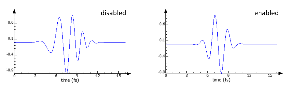
OPTIMIZE FOR SHORT PULSE: Use the shortest possible source pulse.
- This option is enabled by default in the FDTD solver. It should only be disabled when it is necessary to minimize the power injected by the source that is outside of the source range (eg. convergence problems related to broadband steep angled injection).
- This option is disabled by default in the varFDTD solver, as it improves the algorithms numerical stability.
ELIMINATE DC: Eliminates the DC component by forcing signal symmetry

Manual calculation of the source time signal

As explained above, the 'Standard' source type uses a fixed carrier with a gaussian envelope. The following script code shows how to calculate the source time signal used by the source.

# calculate standard pulse time signal
frequency  = 300e12;
pulselength = 50e-15;
offset   = 150e-15;

t      = linspace(0,600e-15, 10000);
w_center  = frequency*2*pi; 
delta_t   = pulselength/(2*sqrt(log(2)));
pulse = sin( -w_center*(t-offset)) * exp( -(t-offset)^2/2/delta_t^2 );

plot(t*1e12,pulse,"t (fs)","source pulse time signal");

Note:

There are some small differences between the pulse generated by this code and the actual time signal generated by the 'standard' source pulse setting. If you need very precise control over or knowledge of the source time signal, you should create your own Custom time signal.

The 'broadband' option is generated with a more complex function. The precise function is not provided. To create your own arbitrary source time signals, see the Custom time signal page.

Beam options tab

In the general tab, set the source shape option to the desired shape (Gaussian, plane wave or Cauchy/Lorentzian) before entering data in the beam options tab because the beam options that are available will change depending on the source shape.

Beam options for all source shapes

THETA VS WAVELENGTH PLOT: This plot shows the actual injection angle theta for each source wavelength as used in the simulation.

Multifrequency beam calculation

MULTIFREQUENCY BEAM CALCULATION checkbox enables/disables the calculation of the source profile at multiple frequency points. This feature is recommended for broadband simulations, and injection in a dispersive material, particularly if injection under an angle is involved. It is important to remember that if this option is not checked, the same spatial field profile at all frequencies is injected. See this dedicated topic for more information about this feature.
NUMBER OF FREQUENCY POINTS specifies how many frequency points are going to be used to compute the field profile.

Beam options for Gaussian and Cauchy/Lorentzian sources

USE SCALAR APPROXIMATION / USE THIN LENS: These checkboxes allow the user to choose whether to use the scalar approximation for the electric field or the thin lens calculation. Gaussian sources can be defined using either the scalar approximation or thin lens calculation, whereas Cauchy/Lorentzian sources can only be defined using the scalar approximation.

VISUALIZE BEAM DATA: This button opens up a visualizer window where you can plot the current calculated beam electric and magnetic field profile over the injection plane.

Scalar approximation (Gaussian and Cauchy/Lorentzian)

BEAM PARAMETERS: This menu is used to choose to define the scalar beam by the WAIST SIZE AND POSITION or the BEAM SIZE AND DIVERGENCE ANGLE.

If WAIST SIZE AND POSITION is chosen, the options are:

WAIST RADIUS: 1/e field (1/e2 power) radius of the beam for a Gaussian beam, or a half-width half-maximum (HWHM) for the Cauchy/Lorentzian beam.
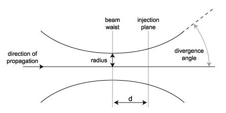
DISTANCE FROM WAIST: The distance, d, as shown in the figure below. A positive distance corresponds to a diverging beam, and a negative sign corresponds to a converging beam.

If BEAM SIZE AND DIVERGENCE ANGLE is chosen, the options are:

BEAM RADIUS: 1/e field (1/e2 power) radius of the beam for a Gaussian beam, or a half-width half-maximum (HWHM) for the Cauchy/Lorentzian beam.
DIVERGENCE ANGLE: Angle of the radiation spread as measured in the far field, as shown in the figure below. A positive angle corresponds to a diverging beam and a negative angle corresponds to a converging beam.

Thin Lens (Gaussian only)

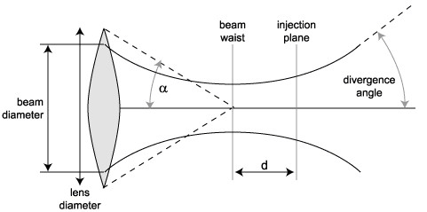
NA: This is n sin(a) where n is the refractive index of the medium in which the source is found and a is the half angle as shown in the figure below. Please note that the index will not be correctly defined in dispersive media and lenses should only be used in non-dispersive media. The refractive index for the source is determined at X, Y (and Z).
DISTANCE FROM FOCUS: The distance d from focus as shown in the figure below. A negative distance indicates a converging beam and a positive distance indicates a diverging beam.
FILL LENS: Checking this box indicates that the lens is illuminated with a plane wave which is clipped at the lens edge. If FILL LENS is unchecked, then it is possible to set the diameter of the thin lens (LENS DIAMETER) and the beam diameter prior to striking the lens (BEAM DIAMETER), as shown in the figure below. A beam diameter much larger than the lens diameter is equivalent to a filled lens.
USE CUSTOM PUPIL FUNCTION: Checking this box applies a pupil (aperture) function to the beam. This option disables the FILL LENS one. The pupil function is defined in direction cosine space (i.e. normalized k-space) by a matrix dataset with parameters u1 and u2 on the plane perpendicular to the injection axis of the source. The matrix dataset must be called "pupil" and it must have either a single scalar attribute named "p" or two scalar attributes named "E1" and "E2"; the second case can be used to modify the polarization of the beam. The matrix dataset can be loaded from a matlab file using the LOAD PUPIL FUNCTION button or from the Lumerical script workspace using the command importdataset. For more information see this example.
NUMBER OF PLANE WAVES: This is the number of plane waves used to construct the beam. The beam profile is more accurate as this number increases but the calculation takes longer. The default value in 2D is 1000.

TIP: selecting the beam option

When the beam waist radius is several times larger than the wavelength used, scalar approximation option should be selected. When the beam waist radius is roughly on the same order as the wavelength, the thin lens option should be used.

Note: References for the thin lens source

The field profiles generated by the thin lens source are described in the following references. For uniform illumination (filled lens), the field distribution is precisely the same as in the papers. For non-uniform illumination at very high NA (numerical aperture), there are some subtle differences. This is due to a slightly different interpretation of whether the incident beam is a Gaussian in real space or in k-space. This difference is rarely of any practical importance because other factors such as the non-ideal lens properties become important at these very high NA systems.

M. Mansuripur, "Distribution of light at and near the focus of high-numerical-aperture objectives," J. Opt. Soc. Am. A 3,2086-2093 (1986).
M. Mansuripur, "Certain computational aspects of vector diffraction problems," J. Opt. Soc. Am. A 6, 786-805 (1989).
M. Mansuripur, "Distribution of light at and near the focus of high-numerical-aperture objectives: erratum, Certain computational aspects of vector diffraction problems: erratum" J. Opt. Soc. Am. A 10, 382-383 (1993).

The figure below shows the beam parameter definitions for the scalar approximation beam.

The figure below shows the beam parameter definitions for the thin lens, fully-vectorial beam.

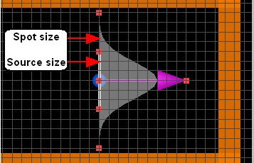
TIP: Setting Gaussian source parameters

Gaussian spot size: The beam spot size can be set independently of the source span. The source span should be chosen to be larger than the beam spot size. If the spot size is larger than the simulation region, the beam profile will be truncated at the simulation boundary. If there is significant intensity at the edges of the source, as shown in this figure, the beam will scatter on injection.

Results returned

FIELDS: The fields injected at the injection plane is returned as a function of position and frequency/wavelength.
INDEX: The index of the region the source covers is returned. This value does not refresh automatically, user needs to re-calculate the FIELDS.
TIME SIGNAL: Time domain signal of the source pulse.
SPECTRUM: The fourier transform of time signal.

Plane wave and beam source - Simulation object