This section describes the power radiated by a dipole in a homogeneous material.
Theoretical power radiated by a dipole in a homogeneous material
The analytic expressions of total radiated power of electric and magnetic dipoles in a homogeneous material of refractive index n, in 2D and 3D are shown in the following table.
| Dipole type | Total radiate power (Watts) | Units |
|---|---|---|
|
2D TM Electric Dipole |
$$ P=\frac{\pi}{2} \frac{\mu_{0}}{4 \pi}\left|\vec{p}_{0}\right|^{2} \omega^{3} $$ |
[p0] = Cm/m |
|
2D TE Electric Dipole |
$$ P=\frac{\pi}{4} \frac{\mu_{0}}{4 \pi}\left|\vec{p}_{0}\right|^{2} \omega^{3} $$ |
[p0] = Cm/m |
|
3D Electric Dipole |
$$ P=\frac{\mu_{0}}{4 \pi} n\left|\vec{p}_{0}\right|^{2} \frac{\omega^{4}}{3 c} $$ |
[p0] = Cm |
|
2D TM Magnetic Dipole |
$$ P=\frac{\pi}{4} \frac{\mu_{0}}{4 \pi} n^{2}\left|\vec{m}_{0}\right|^{2} \frac{\omega^{3}}{c^{2}} $$ |
[m0] = Am2/m |
|
2D TE Magnetic Dipole |
$$ P=\frac{\pi}{2} \frac{\mu_{0}}{4 \pi} n^{2}\left|\vec{m}_{0}\right|^{2} \frac{\omega^{3}}{c^{2}} $$ |
[m0] = Am2/m |
|
3D Magnetic Dipole |
$$ P=\frac{\mu_{0}}{4 \pi} n^{3}\left|\vec{n}_{0}\right|^{2} \frac{\omega^{4}}{3 c^{3}} $$ |
[m0] = Am2 |
Verifying the emitted power in FDTD.
The script file usr_dipole_power.lsf will compare the above analytic formulas for power radiated by a dipole with the measured results from an FDTD simulation. To run this example, download all three assocated files. Open one of the simulation files (.fsp), then run the script.
The script will run a total of 6 simulations, one for each of the dipole type listed above. In each case, it will compare the total measured power in FDTD/Propagator with the analytic expressions. It does this over a wavelength range of 1 to 2 um. It plots both the measured power and the analytical result for each case. The sourcepower function evaluates the analytic expression described above. The dipolepower function measures the actual power radiated by the dipole.
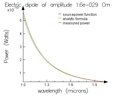
The 3D electric and magnetic dipole comparisons are shown in Figure 1. The percentage difference between the measured result and the analytical expression as a function of points per wavelength in the homogeneous material are shown in Figure 2.

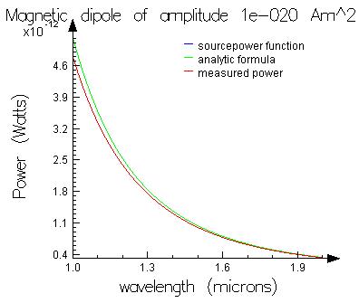
Analytic and measured power for electric and magnetic dipoles.
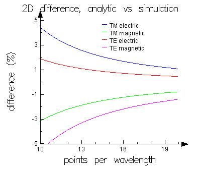
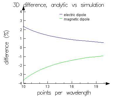
Difference between the analytical power for a dipole and the simulated power in 2D and 3D
(TE/TM and electric/magnetic dipoles).
It is important to understand the following points:
- The main source of the discrepancy is that FDTD is solved on a discrete mesh. The analytic expression comes from a calculation that assumes a continuous homogeneous material instead of a discrete mesh. Therefore it is expected that there is a difference between the simulation and theory which should only go to zero when the mesh size becomes very small.
- In principle, dipole sources are injected by exciting the electric and magnetic fields at only one point on the mesh. In order to allow injection at arbitrary spatial positions and dipole orientations, several mesh points are actually excited with appropriate weighting's. This means that the total injected power changes when you move the dipole by amounts smaller than the mesh size, dx. At 10 points per wavelength, this change in power can be as large as 5% by moving the dipole by dx/2. In Figure 2, the 2D TE electric dipole has the best agreement with the analytic expression compared to the other 2D dipoles, but moving the dipole location by a small amount can make a different dipole type have the best agreement.
We should note that we can compare to the analytic expression for the power radiated from dipoles to within approximately 5% accuracy at 10 points per wavelength. This corresponds to a Mesh Accuracy setting of approximately 2. At 20 points per wavelength (Mesh Accuracy approximately 4-5) the injected power is better than 2%.
The CW normalization option attempts to normalize monitor data to the amount of energy injected into the simulation at each frequency. This allows the user to extract the CW response of a system for a range of frequencies from a single simulation. For this normalization to occur, the injected power must be known. In the case of a dipole, the injected power is calculated from the analytic formula for "total power radiated by a dipole in a homogeneous material".
This means that the simulation data is actually normalized to the amount of power a dipole would inject in a homogenous material, rather than how much power was actually injected into the specific simulation. A dipoles actual injected power can vary significantly from the homogeneous value, depending on what physical structures are near by. Field reflected from nearby structures re-interfere with the source, causing it to inject more or less power than expected. The next section discusses this issue in more detail.