This section applies for FDTD and MODE varFDTD solver, since both use the finite-difference-time-domain method. The simulation files provided in this section are .fsp files, but the same set up can be created using MODE.
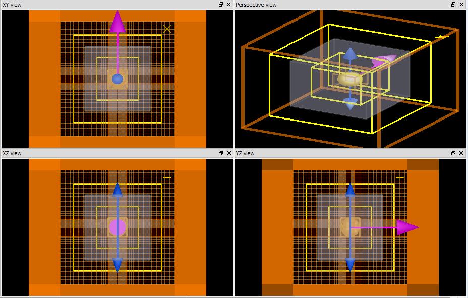
The FDTD algorithm supports a graded mesh of Cartesian (rectangular) cells. This means that the size of the mesh cells can vary as a function of position throughout the simulation region, as shown in the screenshot below. Such a non-uniform mesh can make FDTD calculations more accurate, while requiring less memory and less computation time than a comparable uniform mesh. There are two ways that the non-uniform mesh improves accuracy: through reducing numerical dispersion and improving the resolution of interfaces.
Reduced Numerical Dispersion
Numerical dispersion is an artifact resulting from the discrete spatial sampling of the FDTD mesh. This means that for a coarse mesh, the speed of light on the FDTD mesh may depart slightly from the exact value of the speed of light in the material being simulated. Furthermore, the speed of light becomes slightly anisotropic, in that it depends on the direction of propagation of the light relative to the mesh. The critical parameter that affects numerical dispersion is N = lambda_0/(n D) where lambda_0 is the free space wavelength, n is the refractive index and D is the FDTD mesh cell size. N represents the number of mesh cells per wavelength, and the numerical dispersion artifact becomes negligible as N becomes large. If the refractive index, n, is complex, then both the real and imaginary parts are considered to ensure that it has enough points per wavelength and enough points per decay length for accurate modeling.
The automesh feature automatically configures the non-uniform mesh to minimize the effects of numerical dispersion. In the usual use case, the user simply chooses a setting on the accuracy slider, which ranges in value from 1 to 8. A value of 1 creates a coarse mesh (corresponding to a small N), giving the fastest and lowest memory simulations but also introduces some (several percent) error due to the numerical dispersion artifact. At the other end of the scale, a setting of 8 creates a very fine mesh (N is large), requiring more time and memory, while ensuring that numerical dispersion is a negligible contribution to errors in virtually all situations. Simulation accuracy and computational resource requirements can be traded off in this way. For most applications, a setting of between 2 and 5 on the accuracy slider is sufficiently accurate.
Ability to accurately resolve interfaces
Many optical structures have properties that are critically sensitive to the precise locations of material interfaces. This is particularly true of structures that have resonant characteristics or high index contrast interfaces. The non-uniform mesh makes it possible to take into account the precise geometric location of these interfaces by using fine mesh cells in regions where the interfaces are important and larger mesh cells in bulk regions where there are no important interfaces as with homogeneous materials.
Lumerical provides special mesh objects termed "mesh override" objects that enable the user to indicate where the interfaces are physically significant to the problem. The automesh feature, which otherwise operates as it normally does, will then also take into account the override regions, as well as continuing to reduce numerical dispersion throughout the simulation volume. The mesh override feature is particularly useful for structures with metallic interfaces.