This page explains how conformal mesh technology can be used to improve simulation accuracy and why it is important on a finite sized mesh. For details on how to choose the best mesh refinement option for your application, please see Selecting mesh refinement options.
The conformal mesh method
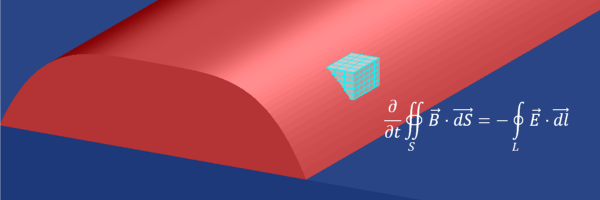
The concept of the conformal mesh is to use an integral solution of Maxwell's equations near interfaces. The method used in Lumerical's software is similar to the methods described in the following publications, with some proprietary modifications:
- Yu, W., and R. Mittra, "A conformal finite difference time domain technique for modeling curved dielectric surfaces," IEEE Microwave Components Lett,, Vol. 11, 2001, pp. 25-27.
- Allen Taflove, Computational Electromagnetics: The Finite-Difference Time-Domain Method. Boston: Artech House, (2005).
- Y. Zhao and Y. Hao, “Finite-difference time-domain study of guided modes in nano-plasmonic waveguides,” IEEE Trans. Antennas Propag. 55, 3070–3077 (2007).
- A. Mohammadi, H. Nadgaran, and M. Agio, “Contour-path effective permittivities for the two dimensional finite-difference time-domain method,” Opt. Express 13, 10367–10381 (2005) .
Mesh refinement choices
To enable conformal meshing, go to the Simulation Region "Mesh settings" tab.
Please see Mesh refinement options for details on how to choose the conformal mesh settings for your application.
Maxwell's equation on a finite mesh
There are two key challenges associated with solving Maxwell's equations on a finite mesh:
- There are numerical errors associated with the finite mesh size, even in homogenous material. For example, the speed of light on a finite mesh is not the same as real space, but depends on dx, dy, dz and dt. Lumerical's graded meshing with automatic mesh generation solves this problem by adjusting the mesh to the refractive index of the materials. For example, the mesh in a material of n=2 will be twice as small as in a material with n=1, because the wavelength is smaller in the higher index material. This ensures that the numerical errors associated with the finite mesh are kept below a certain threshold in all regions of the simulation.
- It is not possible to resolve interfaces to higher precision than the size of the mesh used. One solution is to use mesh override regions to force a very small spatial mesh near interfaces. The disadvantage of this method is that it can greatly increase simulation times and memory requirements. In the FDTD method, the simulation time scales as 1/dx^4 for 3D simulations. A better solution for many applications is to use conformal mesh technology. In some cases, a combination of both solutions is required. In general, we recommend using conformal meshing as much as possible, and sometimes mesh override regions to force a smaller mesh size in critical regions.
The default conformal setting will apply conformal meshing to all materials except metals and PEC. Please see Mesh refinement options for a detailed description of the different mesh refinement options and how to choose the right setting for your application.
The figures below shows some typical structures where problems with a finite mesh size are encountered.
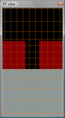
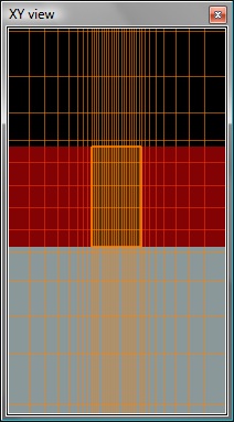
Example 1
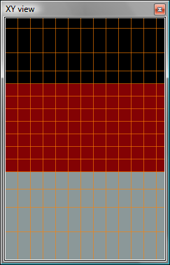

Default mesh, Graded mesh
A 50nm thick layer of silicon on glass. The simulation mesh size is approximately 7nm. Without conformal meshing, the layer thickness cannot be defined to better than 7nm - in other words, a 49nm layer and a 55nm layer can give exactly the same results!
The graded mesh solution uses mesh override regions to make the mesh size 1nm at the interfaces, however many more mesh points are needed. The conformal mesh solution allows you to obtain accurate results for this type of structure without using any mesh override regions. Please note that you should see at least 2 mesh cells in your layer.
Example 2
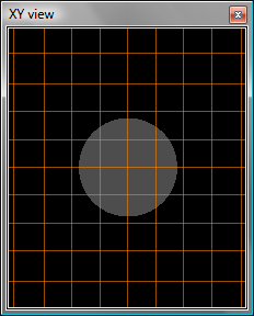
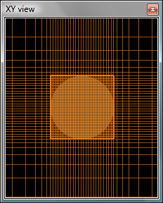
Default mesh, Graded mesh
A silver rod of diameter 50nm. In the default mesh, the curved interfaces cannot be well resolved. The graded mesh solution forces a much smaller mesh over the entire rod, introducing many more grid points.
In this application, we use a combination of graded meshing and conformal meshing. The conformal meshing can allow you to obtain more accurate results for a given mesh size. Even if the mesh size is only twice as large, for example 2nm compared to 1nm, the computation time in 3D simulations can be reduced by a factor of 16. Please take care when using conformal mesh technology with metals, however, and do some convergence testing to be sure that the conformal mesh technology is appropriate for your precise application.
Example 3
Default mesh, Graded mesh
A waveguide coupler region made from two silicon waveguides a short distance apart. The coupling length is critically sensitive to the distance between the waveguides, which can't be resolved to better than the size of dx without conformal mesh technology.
The graded mesh solution forces a much smaller mesh between the waveguides, in order to resolve the distance to any desired accuracy.
The conformal mesh solution will allow you to obtain accurate results for this type of structure without using a special mesh override region between the waveguides. Please note that the space between the waveguides should be at least 2*dx. If this is not the case, a mesh override region may be necessary to ensure this, even with the conformal mesh.
Simulation times and memory requirements
The following table shows the relationship between mesh step size and simulation time and memory requirements for 2D and 3D simulations:
|
3D |
2D |
|
|
Memory requirements |
\( \sim V(\lambda /dx)^3 \) |
\( \sim A(\lambda /dx)^2 \) |
|
Simulation time |
\( \sim V(\lambda/dx)^4 \) |
\( \sim A(\lambda /dx)^3 \) |