Motivation
This topic describes how to use a parameter sweep in MODE to do dispersion calculations much like those available in the frequency analysis tab of the Eigensolver. While the GUI allows for easy and quick setup of a frequency sweep, the parameter sweep will achieve the same results with more versatility. Here, we sweep over frequency to generate the same plots of dispersion, neff, group velocity, etc. This technique can be generalized to sweep over any other parameter and generate plots of other figures of merit in other Lumerical’s products.
Another advantage of using this technique is that the multiple simulations in a sweep can be distributed to yield faster results for larger simulation files.
Simulation setup
The structure we will be considering is a silicon waveguide embedded in SiO2 cladding. The "sweep" object in the Optimization and Sweeps window performs a sweep over a frequency range of 193 - 200 THz (1.5 - 1.55 um).
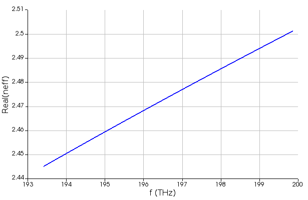
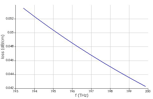
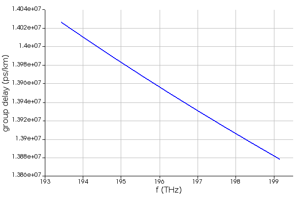
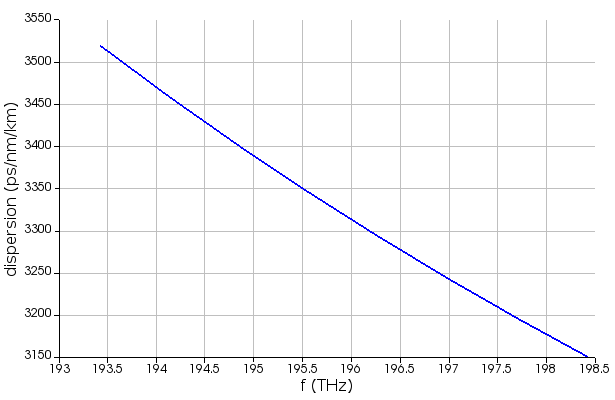
We will first track the fundamental TE mode of the waveguide, and calculate its various modal properties including the dispersion. When calculating a result involving derivatives of the refractive index, discontinuities in the refractive index data can cause artificial discontinuities in the resulting plots. To avoid such issues, it is recommended to enable the multi-coefficient material fittings in the Material Explorer.
Run and Results
- Open the script file, sweep_frequency_dispersion.lsf, in MODE.
- Modify the input parameters such as start/stop frequencies and run the script.
Since the purpose of this example is to replicate what is done in the "Frequency analysis" tab, we use the same input parameters as in the GUI. Note that the start and stop frequencies in the "sweep" object are automatically set up based on the values you specify in the script file.
If the "track_selected_mode" variable is set to "1", the sweep will run the simulation for the first frequency and set the desired mode as a reference dcard. Then as the frequency is swept the overlap between the selected dcard and the corresponding mode at the new frequency is used to track that mode. The differences here with the frequency analysis of the user interface are as follows:
- The sweep is first completed over the frequency points specified, resulting in the same number of sweep files saved.
- The individual sweep files are sequentially loaded and the figures of merit are calculated afterward.
Once the sweep is completed, the following plots are generated: