In this article we will discuss how the source fields are rotated into an appropriate local coordinate- system \( \mathbf{ \hat{e}_L} \) from the global cartesian system \( \mathbf{\hat{e}_G} \) and vice versa. In the local coordinate system of the source, k -the wave vector- will be purely along \( \hat{z} \) and the fields will be in the \( \hat{x} \text{, } \hat{y} \) plane depending on the polarization angle. The global coordinate system is apparent from the CAD view window and consistent across all simulations no matter the incidence angle specified.
$$ \mathbf{ \hat{e}_L} \overset{A(\theta)}{\longrightarrow} \mathbf{ \hat{e}_\theta} \overset{B(\phi)}{\longrightarrow} \mathbf{ \hat{e}_\phi} \overset{C(ia)}{\longrightarrow} \mathbf{\hat{e}_G} $$
$$ \left(\begin{array}{c} x'\\ y'\\ z'\end{array}\right) \to \left(\begin{array}{c} x''\\ y''\\ z''\end{array}\right) \to \left(\begin{array}{c} x'''\\ y'''\\ z'''\end{array}\right) \to \left(\begin{array}{c} x\\ y\\ z\end{array}\right) $$
To achieve the required injection angle three different rotations around predefined axes can be used, for more information on rotation formalism in 3D see this page. In FDTD we have chosen achieve this coordinate transformation using two angles \( \theta \) and \( \phi \) , as well giving the user the choice of specifying the injection axis in \( \mathbf{\hat{e}_G} \) . Even with this knowledge the actual rotation matrix is not unique and so here we will share explicitly the transformation procedure. In the vast majority situations, it is unnecessary to work out the transformation yourself, and it should be sufficient to simply look at the GUI. In optics understanding the sources coordinate system may be useful when one is working with S, and P waves in the plane of incidence, or post process the results of the far-field projection. Typically users will have to work out additional transformations based on their choice of coordinate system, but if you understand how to move from \( \mathbf{\hat{e}_G} \) -> \( \mathbf{ \hat{e}_L} \) this should be possible. When comparing field components one must be careful as the polarity of the basis can cause an unexpected \(\pi\) phase shift; this is apparent in different sign conventions for the Fresenel coefficients for example.
Our approach here is to give an intuitive explanation and provide all the necessary mathematics required to work out the rotation matrices. These are not explicitly provided but can be calculated by multiplying the appropriate matrices together in the correct order. To make this simple we will work from the local coordinate system \( \mathbf{ \hat{e}_L} \) through each rotation until we reach \( \mathbf{ \hat{e}_G} \). Working from \( \mathbf{ \hat{e}_G} \) -> \( \mathbf{ \hat{e}_L} \) is harder to follow in general, but we will show that you get this inverse rotation \( \mathbf{ \hat{e}_L} \) -> \( \mathbf{ \hat{e}_G} \) for free using some linear algebra identities.
Polarization
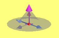
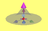
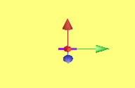
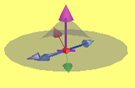
The polarization matrix is not precisely part of the coordinate transformation; however, it is important as it rotates the fields in the beams coordinate system. This allows any combination of E field and k vector to be achieved and will be visible in the GUI as the arrow of the source. Initially in \( \mathbf{ \hat{e}_L} \) the E field will be purely polarized along \( \hat{x}' \). Hence a polarization angle \( \psi = 0 \) will leave the fields unchanged as P reduces to an identity rotation matrix. A polarization angle \( \psi = 90 \) degrees will rotate the fields so that E is || \( \hat{y}' \).
$$ P = \left( \begin{array}{ccc }{\cos(\psi)} & {-\sin(\psi)} & {0} \\ {\sin(\psi)} & {\cos(\psi)} & {0} \\ {0} & {0} & {1} \end{array} \right) $$
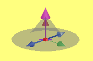
Pol = 0
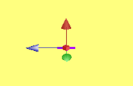
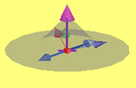
Pol = 90
Pol=45
Theta
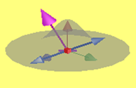
Theta corresponds to a rotation about the \( \hat{y}' \). This will change the incidence angle of the beam by rotating k which is initially aligned with \( \hat{z}' \) (red). Theta can take on values of -89.9 < \(\theta\) < 89.9.
$$ A(\theta) = \left( \begin{array}{ccc }{\cos(\theta)} & {0} & {\sin(\theta)} \\ {0} & {1} & {0} \\ {-\sin(\theta)}& {0} & {\cos(\theta)} \end{array} \right) $$
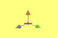
Theta = 0
Theta = 45
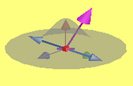
Theta = -45
Phi
If \(\theta \neq 0 \) the \(\phi\) angle rotates around the intermediate \( \hat{z}'' \) in a reference frame we refer to as \( \mathbf{ \hat{e}_\theta} \). If \(\theta = 0 \) then \( \hat{z}' = \hat{z}'' = \hat{z}''' \) and \( B(\phi) \) operates in the exact same way as \(P(\psi) \), the polarization rotation, except that it is operating on the coordinates and not the field components.
$$ B(\phi) = \left( \begin{array}{ccc }{\cos(\phi)} & {-\sin(\phi)} & {0} \\ {\sin(\phi)} & {\cos(\phi)} & {0} \\ {0} & {0} & {1} \end{array} \right) $$
Theta=0, Phi = 45
Theta = 0, Phi = -45
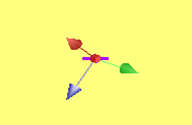
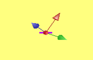
As you can see given if \(\theta = -25 \) degrees and \( \phi = -45 \text{, } 135 \) the \( \hat{z}''' \) axis is tilted relative to the initial k by \(\theta\) and \( \hat{x}''', \hat{y}''' \) are rotated by \( \phi\). Notice that from the perspective of the new coordinates this has the effect of rotating the k vector about \( \hat{z}''' \). Let us call this new coordinate system \( \mathbf{ \hat{e}_\phi} \).
At this point we should note that we have essentially transformed into the global coordinate system \( \mathbf{ \hat{e}_G} \) from \( \mathbf{ \hat{e}_L} \) up to a permutation of the axes based on the chosen injection axes.
From \( \mathbf{ \hat{e}_\theta} \), where \( \theta = 25\), and \(\phi = -45 \).
From \( \mathbf{ \hat{e}_\phi} \), where \( \theta = 25 \), and \(\phi = -45\).
From \( \mathbf{ \hat{e}_\theta} \), where \( \theta = 25\), and \( \phi = 135\).
From \( \mathbf{ \hat{e}_\phi} \), where \( \theta = 25 \), and \( \phi = 135 \).
Injection axis
The injection axis rotation allows you to permute the axes to achieve the desired injection angle. That is the coordinates are changed so that if \(\theta \), and \( \phi = 0\) then \( \hat{z}'\) would be || to the specified direction and axis.
$$ \hat{x} : C(ia) =\left(\begin{array}{ccc} 0 & 0 & 1 \\ 1 & 0 & 0 \\ 0 & 1 & 0\end{array}\right)$$
$$ \hat{y} : C(ia) =\left(\begin{array}{ccc} 0 & 1 & 0 \\ 0 & 0 & 1 \\ 1 & 0 & 0\end{array}\right)$$
$$ \hat{z} : C(ia) =\left( \begin{array}{ccc} 1 & 0 & 0 \\ 0 & 1 & 0 \\ 0 & 0 & 1 \end{array} \right)$$
For a surface with normal either parallel to the specified injection axis, and k you have defined the plane of incidence with polarization automatically in plane for zero polarization angle. Therefore to get P, and S polarized light it is sufficient to specify a polarization angle \(\psi = 0\text{, } 90\) degrees respectively.
Injection Direction
For forward propagation there is nothing else to consider. This section outlines the additional steps taken to define the E fields and k vector of backwards propagating source.
If the injection direction is set to backwards the same coordinate transform C, defined above, is used for the fields. The difference is that in the original reference frame the E field profile is conjugated.
$$ \mathbf{E} \to \mathbf{E}^* $$
The k vector is then reflected about the origin by negating each component. This is only applied to the k vector and not the fields.
$$ -\hat{x} : C=\left( \begin{array}{ccc} 0 & 0 & -1 \\ -1 & 0 & 0 \\ 0 & -1 & 0\end{array} \right)$$
$$ -\hat{y} : C=\left( \begin{array}{ccc} 0 & -1 & 0 \\ 0 & 0 & -1 \\ -1 & 0 & 0\end{array} \right)$$
$$ -\hat{z} : C=\left( \begin{array}{ccc} -1 & 0 & 0 \\ 0 & -1 & 0 \\ 0 & 0 & -1\end{array} \right)$$
H fields
The H fields are readily calculated using Maxwell’s curl equation in frequency domain. Once the E field has been rotated through P and conjugated if the direction is backwards, the H fields are calculated as so.
$$ \mathrm{FT}\{\nabla \times \boldsymbol{E}=\boldsymbol{d} \boldsymbol{B} / \boldsymbol{d} \boldsymbol{t}\} \Rightarrow \nabla \times \boldsymbol{E}=-i \omega \mu \boldsymbol{H} $$
For a plane wave with polarization angle zero and forward propagation direction this reduces to
$$\left|\begin{array}{ccc} \hat{x}' & \hat{y}' & \hat{z}' \\ \frac{\partial}{\partial x} & \frac{\partial}{\partial y} & \frac{\partial}{\partial z} \\ E_{x} & 0 & 0\end{array}\right|=-i \omega \mu \boldsymbol{H}$$
$$-i \omega \mu\left(\frac{\partial E_x}{\partial z} \hat{y}'\right)=-i \omega \mu(H_y \hat{y}' )$$
Inverse Rotation
With the three rotation transformations defined above we have shown how to transform the coordinates from the local reference frame of the source \( \mathbf{ \hat{e}_L} \) to the global coordinates \( \mathbf{ \hat{e}_G} \). Fortunately this allows us to immediately define the inverse transformation from the source fields given in \( \mathbf{ \hat{e}_G} \), back to the initial reference frame.
The transformation we have described can be represented as the product of \( A(\theta), B(\phi), and C(ia) \). It is important to remember that matrix multiplication is not commutative so the ordering is essential. Remember A was multiplied first, then B and then C. The upshot is that you can use a single transformation which is the product of the above rotations
$$ \mathbf{ \hat{e}_G }= C(ia) B(\phi)A(\theta) \mathbf{ \hat{e}_L} = D(\theta,\phi,ia) \mathbf{ \hat{e}_L} $$
Using the following linear algebra identities and properties of orthogonal matrices we obtain the inverse transformation expressed as either the transpose of the product or product of the transposes.
Orthogonal matrices: \( A^{-1} = A^T \)
Transpose property: \( (AB)^T = B^T A^T \)
$$ \mathbf{ \hat{e}_L }= D^T \mathbf{ \hat{e}_G }= A(\theta)^T B(\phi) ^T C(ia)^T \mathbf{ \hat{e}_G } $$
Finally the polarization will operate on the fields first in the transformation we outlined and last in the inverse transformation.
$$ \mathbf{ \hat{e}_G }= D P \mathbf{ \hat{e}_L} $$
$$ \mathbf{ \hat{e}_L }= P^T D^T \mathbf{ \hat{e}_G} $$